import numpy as np
import matplotlib.pyplot as plt
import torch
import torch.nn as nn
import torch.nn.functional as F
from torch.utils.data import TensorDataset, DataLoader
from sklearn.datasets import load_digits
from sklearn.model_selection import train_test_split

# Set random seeds for reproducibility
torch.manual_seed(42)
np.random.seed(42)

# Use GPU if available
device = torch.device("cuda" if torch.cuda.is_available() else "cpu")
print(f"Using device: {device}")Autoencoders from First Principles: Intuition, Mathematics, and PyTorch
A beginner-friendly journey through compression, reconstruction, probabilistic thinking, and hands-on implementation
Deep Learning
Representation Learning
PyTorch
Tutorial
Representation Learning
Autoencoders from First Principles
Have you ever wondered how Netflix compresses movies, or how your brain remembers faces without storing every pixel? Autoencoders learn to do something similar: they find the essential information in data and throw away the rest. In this tutorial, we build that understanding step by step—starting from everyday intuition, moving through the mathematics, exploring a probabilistic perspective, and finishing with a working PyTorch implementation.
What You Will Learn
By the end of this blog, you will be able to:
- Explain what an autoencoder does in plain English
- Write down the mathematical objective and interpret every symbol
- Calculate a toy example by hand (with numbers!)
- Understand why MSE loss has a probabilistic meaning
- Distinguish between vanilla, sparse, denoising, and variational autoencoders
- Implement a working autoencoder in PyTorch from scratch
Part 1: Building Intuition
Before we write any equations, let us build a mental picture of what autoencoders are trying to do.
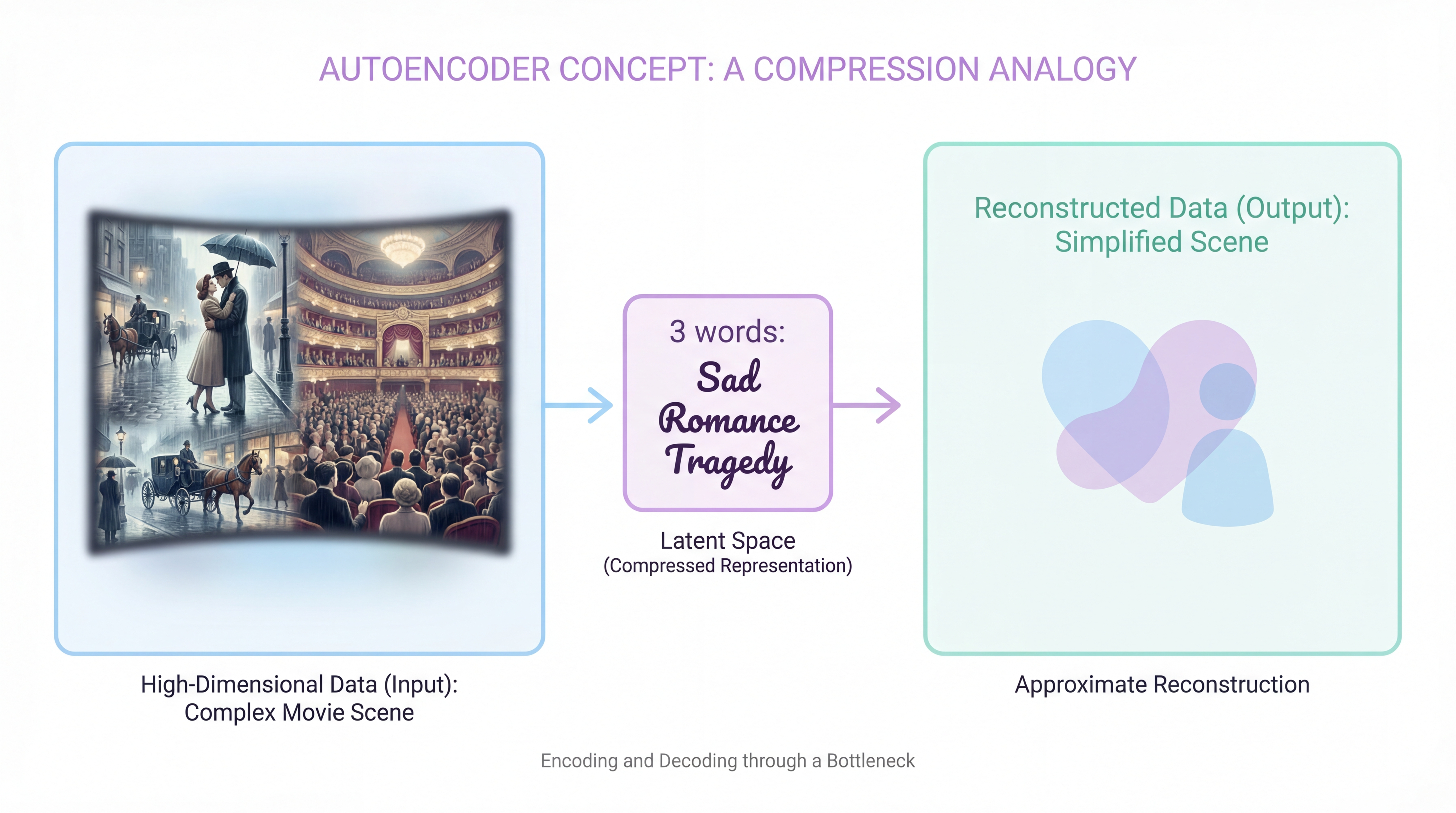
The Compression Analogy
Imagine you have a friend who lives far away, and you can only send them one letter per week. Each letter can hold exactly 3 words. Your task: describe a movie you watched.
Obviously, you cannot write the entire script. Instead, you must:
- Extract the most important details (genre, main emotion, ending type)
- Compress them into 3 words: “Sad romance tragedy”
- Hope your friend can reconstruct a rough sense of the movie from those 3 words
This is exactly what an autoencoder does:
- Encoder = your brain extracting the 3 key words
- Latent code = the 3-word summary
- Decoder = your friend’s brain reconstructing the movie from the summary
Key Insight
The autoencoder is forced to learn what matters because it has limited space. If we gave you 1000 words, you might copy the script. With only 3 words, you must be clever.
What Problem Are We Actually Solving?
In machine learning, we often deal with high-dimensional data:
| Data Type | Dimensions | Example |
|---|---|---|
| Grayscale image (28×28) | 784 | MNIST digit |
| Color image (64×64) | 12,288 | Face photo |
| Audio clip (1 second) | 44,100 | Speech sample |
| Word embedding | 300 | Word2Vec vector |
But here is the key observation: most of these dimensions are redundant.
- In an image of a “3”, the pixels are highly correlated (the top loop connects to the bottom loop)
- In speech, neighboring samples are almost the same (smooth waveform)
- In text embeddings, similar words have similar vectors
An autoencoder tries to find this hidden low-dimensional structure and use it to reconstruct the input.
One Sentence Summary
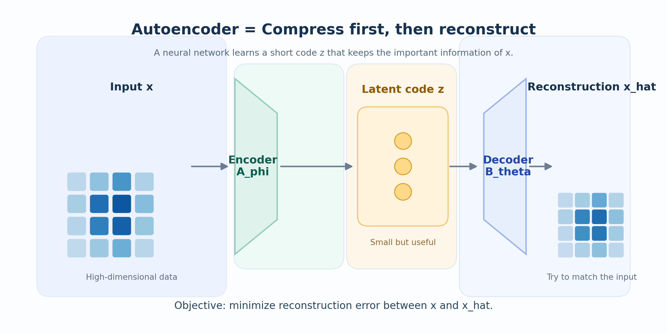
An autoencoder is a neural network trained to reconstruct its own input through a compressed hidden representation.
Part 2: The Mathematical Framework
Now let us write down the mathematics, symbol by symbol.
Step 1: Define the Input
Let the input be a vector:
\[ \mathbf{x} \in \mathbb{R}^n \]
What this means:
- \(\mathbf{x}\) is a single data point (one image, one audio clip, etc.)
- \(\mathbb{R}^n\) means it has \(n\) real-valued components
- Example: for an 8×8 grayscale image, \(n = 64\)
Step 2: Define the Encoder
The encoder is a function that compresses \(\mathbf{x}\) into a smaller code:
\[ \mathbf{z} = f_\phi(\mathbf{x}) \]
where:
- \(f_\phi : \mathbb{R}^n \to \mathbb{R}^p\) is the encoder function
- \(\phi\) represents all the encoder’s learnable parameters (weights and biases)
- \(\mathbf{z} \in \mathbb{R}^p\) is the latent code (also called the bottleneck)
- Crucially: \(p < n\) (the code is smaller than the input)
Why \(p < n\)?
If \(p \geq n\), the encoder could just copy the input directly. The bottleneck forces the encoder to learn meaningful compression.
Step 3: Define the Decoder
The decoder takes the code and tries to reconstruct the original input:
\[ \hat{\mathbf{x}} = g_\theta(\mathbf{z}) = g_\theta(f_\phi(\mathbf{x})) \]
where:
- \(g_\theta : \mathbb{R}^p \to \mathbb{R}^n\) is the decoder function
- \(\theta\) represents the decoder’s learnable parameters
- \(\hat{\mathbf{x}}\) is the reconstruction (our attempt to recover \(\mathbf{x}\))
Step 4: Define the Loss Function
How do we measure if the reconstruction is good? We use a reconstruction loss:
\[ \mathcal{L}(\mathbf{x}, \hat{\mathbf{x}}) = \|\mathbf{x} - \hat{\mathbf{x}}\|_2^2 = \sum_{i=1}^{n} (x_i - \hat{x}_i)^2 \]
In words: We square the difference for each dimension, then sum them up. This is called Mean Squared Error (MSE) or L2 loss.
Step 5: The Full Optimization Problem
Given a dataset \(\{\mathbf{x}^{(1)}, \mathbf{x}^{(2)}, \ldots, \mathbf{x}^{(N)}\}\), we want to find the best encoder and decoder:
\[ \boxed{ (\phi^*, \theta^*) = \arg\min_{\phi, \theta} \frac{1}{N} \sum_{i=1}^{N} \|\mathbf{x}^{(i)} - g_\theta(f_\phi(\mathbf{x}^{(i)}))\|_2^2 } \]
Reading this equation:
- \(\arg\min_{\phi, \theta}\) = “find the values of \(\phi\) and \(\theta\) that minimize…”
- \(\frac{1}{N} \sum_{i=1}^{N}\) = “average over all \(N\) training examples…”
- \(\|\mathbf{x}^{(i)} - g_\theta(f_\phi(\mathbf{x}^{(i)}))\|_2^2\) = “…the squared reconstruction error”
The Core Idea in One Line
The autoencoder asks: What is the smallest code that still lets me rebuild the input well?
Part 3: A Toy Example You Can Calculate by Hand
Let us make this concrete with the simplest possible example.
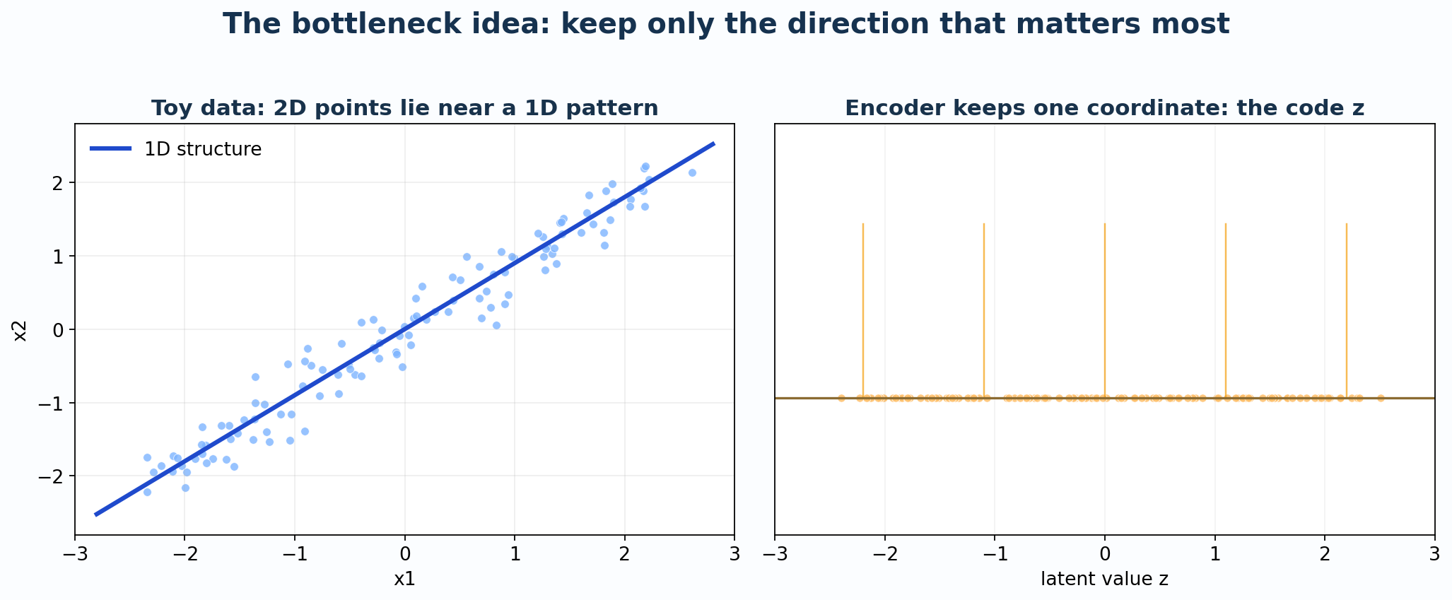
Setup: 2D Data Near a Line
Suppose our data lives in 2D (\(n = 2\)), but it lies near a line:
\[ x_2 \approx 0.9 \cdot x_1 \]
This means the data is technically 2D, but its intrinsic dimensionality is 1D.
A Linear Autoencoder
For this toy case, let us use the simplest possible encoder and decoder:
Encoder (2D → 1D): \[ z = \mathbf{w}^\top \mathbf{x} = w_1 x_1 + w_2 x_2 \]
Decoder (1D → 2D): \[ \hat{\mathbf{x}} = z \cdot \mathbf{v} = z \begin{bmatrix} v_1 \\ v_2 \end{bmatrix} \]
For the line \(x_2 = 0.9 x_1\), a natural choice is:
\[ \mathbf{v} = \begin{bmatrix} 1 \\ 0.9 \end{bmatrix}, \qquad \mathbf{w} = \frac{1}{1 + 0.9^2} \begin{bmatrix} 1 \\ 0.9 \end{bmatrix} = \frac{1}{1.81} \begin{bmatrix} 1 \\ 0.9 \end{bmatrix} \]
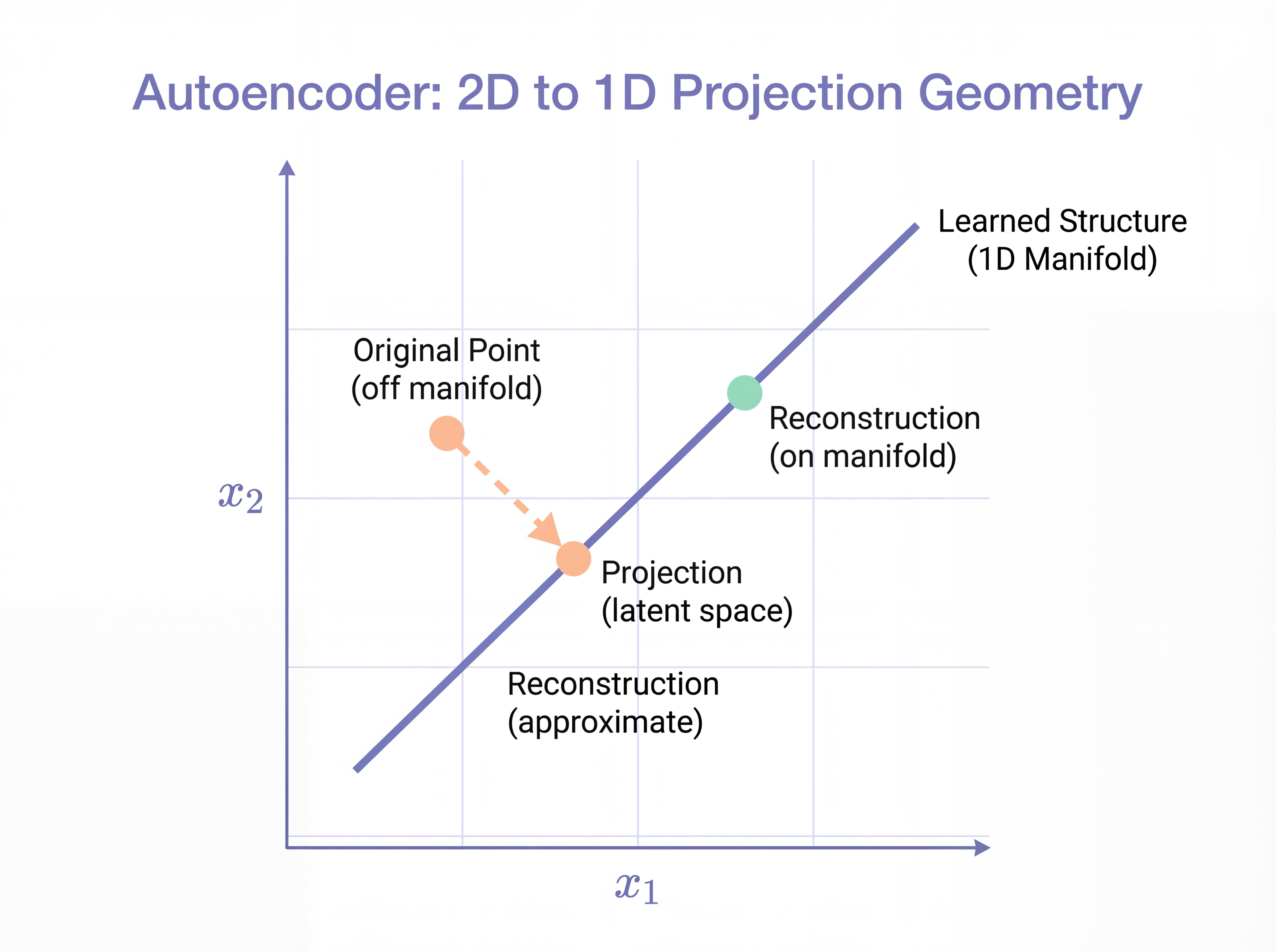
This is the orthogonal projection onto the line.
Worked Example 1: A Point on the Line
Take \(\mathbf{x} = \begin{bmatrix} 2.0 \\ 1.8 \end{bmatrix}\). This point is exactly on the line (since \(1.8 = 0.9 \times 2.0\)).
Step 1: Encode \[ z = \frac{1}{1.81}(1 \cdot 2.0 + 0.9 \cdot 1.8) = \frac{2.0 + 1.62}{1.81} = \frac{3.62}{1.81} = 2.0 \]
Step 2: Decode \[ \hat{\mathbf{x}} = 2.0 \times \begin{bmatrix} 1 \\ 0.9 \end{bmatrix} = \begin{bmatrix} 2.0 \\ 1.8 \end{bmatrix} \]
Result: Perfect reconstruction! The point on the line is recovered exactly.
Worked Example 2: A Noisy Point Off the Line
Take \(\mathbf{x} = \begin{bmatrix} 2.0 \\ 2.4 \end{bmatrix}\). This point is off the line (since \(2.4 \neq 0.9 \times 2.0 = 1.8\)).
Step 1: Encode \[ z = \frac{1}{1.81}(1 \cdot 2.0 + 0.9 \cdot 2.4) = \frac{2.0 + 2.16}{1.81} = \frac{4.16}{1.81} \approx 2.298 \]
Step 2: Decode \[ \hat{\mathbf{x}} = 2.298 \times \begin{bmatrix} 1 \\ 0.9 \end{bmatrix} = \begin{bmatrix} 2.298 \\ 2.068 \end{bmatrix} \]
Step 3: Calculate Error \[ \|\mathbf{x} - \hat{\mathbf{x}}\|^2 = (2.0 - 2.298)^2 + (2.4 - 2.068)^2 = 0.089 + 0.110 = 0.199 \]
Result: The reconstruction is pulled back toward the line. The autoencoder keeps the main structure and discards the noise!
Connection to PCA
If the encoder and decoder are linear (no activation functions), then:
\[ \text{Autoencoder} \approx \text{Principal Component Analysis (PCA)} \]
Both find the principal subspace that captures the most variance in the data.
The difference is:
- PCA: Closed-form solution using eigenvalue decomposition
- Autoencoder: Iterative solution using gradient descent (but can add nonlinearity!)
Part 4: The Probabilistic Perspective
Here is where things get interesting. Let us give the reconstruction loss a probabilistic interpretation.
Viewing the Decoder as a Probability Model
Instead of thinking “the decoder outputs a point \(\hat{\mathbf{x}}\)”, think:
The decoder defines a probability distribution over possible reconstructions.
Specifically, assume:
\[ p_\theta(\mathbf{x} \mid \mathbf{z}) = \mathcal{N}(\mathbf{x}; g_\theta(\mathbf{z}), \sigma^2 \mathbf{I}) \]
In words:
- Given the latent code \(\mathbf{z}\), the decoder says “I think \(\mathbf{x}\) is normally distributed”
- The mean of this distribution is \(g_\theta(\mathbf{z})\) (the decoder’s output)
- The variance is \(\sigma^2\) in every dimension (assumed equal for simplicity)
MSE = Negative Log-Likelihood
The probability density function of a Gaussian is:
\[ p_\theta(\mathbf{x} \mid \mathbf{z}) = \frac{1}{(2\pi\sigma^2)^{n/2}} \exp\left(-\frac{\|\mathbf{x} - g_\theta(\mathbf{z})\|^2}{2\sigma^2}\right) \]
Taking the negative log:
\[ -\log p_\theta(\mathbf{x} \mid \mathbf{z}) = \frac{1}{2\sigma^2} \|\mathbf{x} - g_\theta(\mathbf{z})\|^2 + \underbrace{\frac{n}{2}\log(2\pi\sigma^2)}_{\text{constant}} \]
Key Result: MSE Has a Probabilistic Meaning
Minimizing MSE reconstruction loss is equivalent to maximizing the log-likelihood under a Gaussian decoder model:
\[ \min_{\phi, \theta} \text{MSE} \iff \max_{\phi, \theta} \log p_\theta(\mathbf{x} \mid f_\phi(\mathbf{x})) \]
This is why MSE is the natural loss for continuous data!
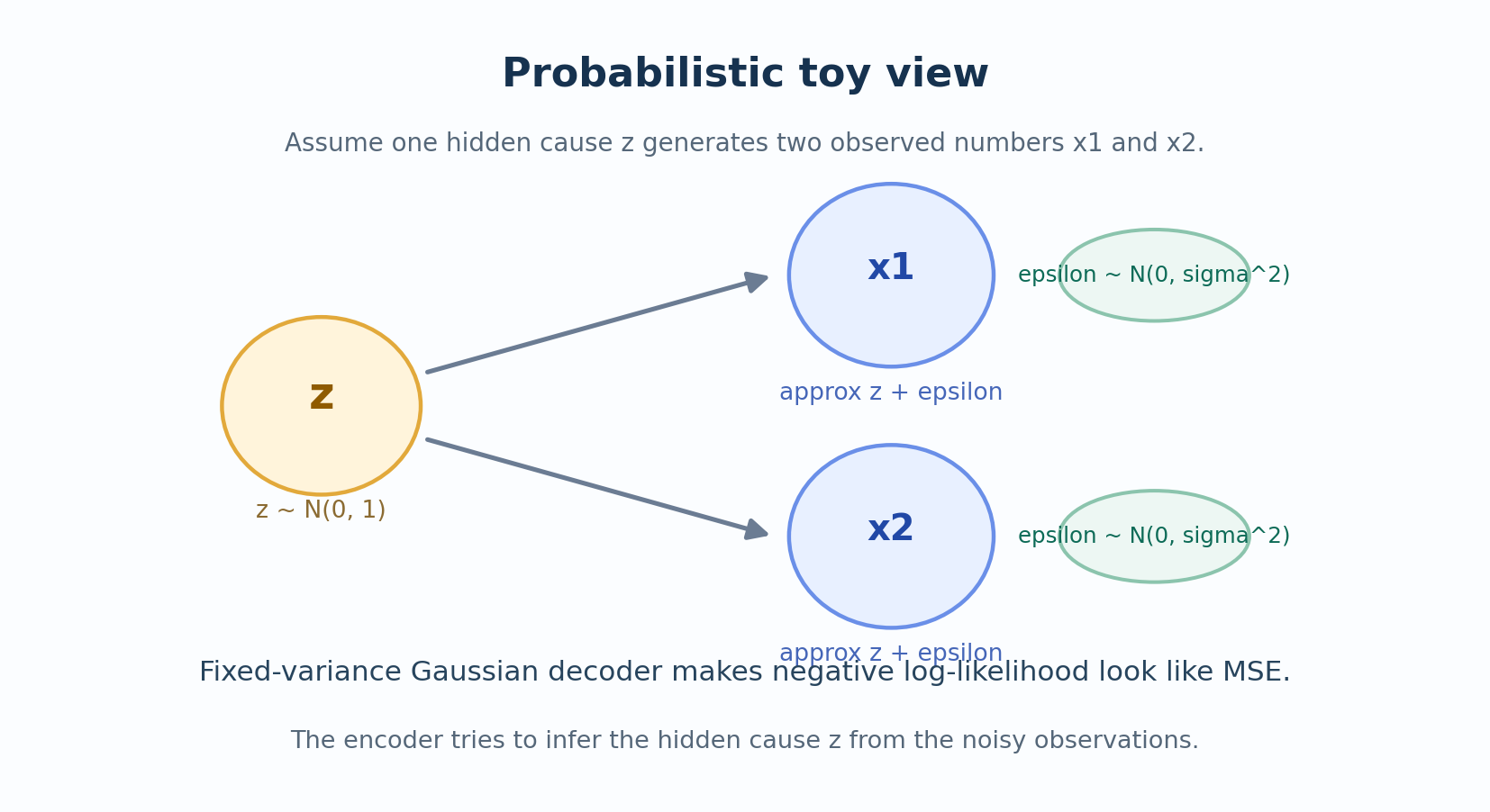
A Toy Probabilistic Example
Let us build a probabilistic toy case from scratch.
The Generative Story
Suppose there is a hidden cause \(z\) that generates two noisy observations:
\[ x_1 = z + \epsilon_1, \qquad x_2 = z + \epsilon_2 \]
where:
\[ z \sim \mathcal{N}(0, 1), \qquad \epsilon_1, \epsilon_2 \sim \mathcal{N}(0, \sigma^2) \text{ (independent)} \]
In words: There is one underlying “truth” \(z\), and we observe two noisy measurements of it.
The Inference Problem
Given observations \((x_1, x_2)\), what is the best estimate of \(z\)?
Likelihood: \[ p(x_1, x_2 \mid z) = \mathcal{N}(x_1; z, \sigma^2) \cdot \mathcal{N}(x_2; z, \sigma^2) \]
Maximum Likelihood Estimate: Taking the derivative and setting to zero, we get:
\[ \hat{z}_{\text{MLE}} = \frac{x_1 + x_2}{2} \]
The best estimate is simply the average of the observations!
Worked Example: Probabilistic Inference
Suppose we observe \(x_1 = 1.2\) and \(x_2 = 0.8\) with noise \(\sigma^2 = 0.5\).
Step 1: Estimate the latent variable \[ \hat{z} = \frac{1.2 + 0.8}{2} = 1.0 \]
Step 2: Reconstruct the observations \[ \hat{x}_1 = \hat{z} = 1.0, \qquad \hat{x}_2 = \hat{z} = 1.0 \]
Step 3: Interpret - Original: \((1.2, 0.8)\) — two noisy measurements - Reconstruction: \((1.0, 1.0)\) — denoised estimate of the true signal
The “autoencoder” here found the hidden factor and used it to denoise both observations!
What This Teaches Us
This toy model captures the essence of what autoencoders do:
- Encoder = infers the hidden cause from observations
- Latent code = the estimated hidden cause
- Decoder = generates reconstructions from the hidden cause
The autoencoder is doing approximate probabilistic inference!
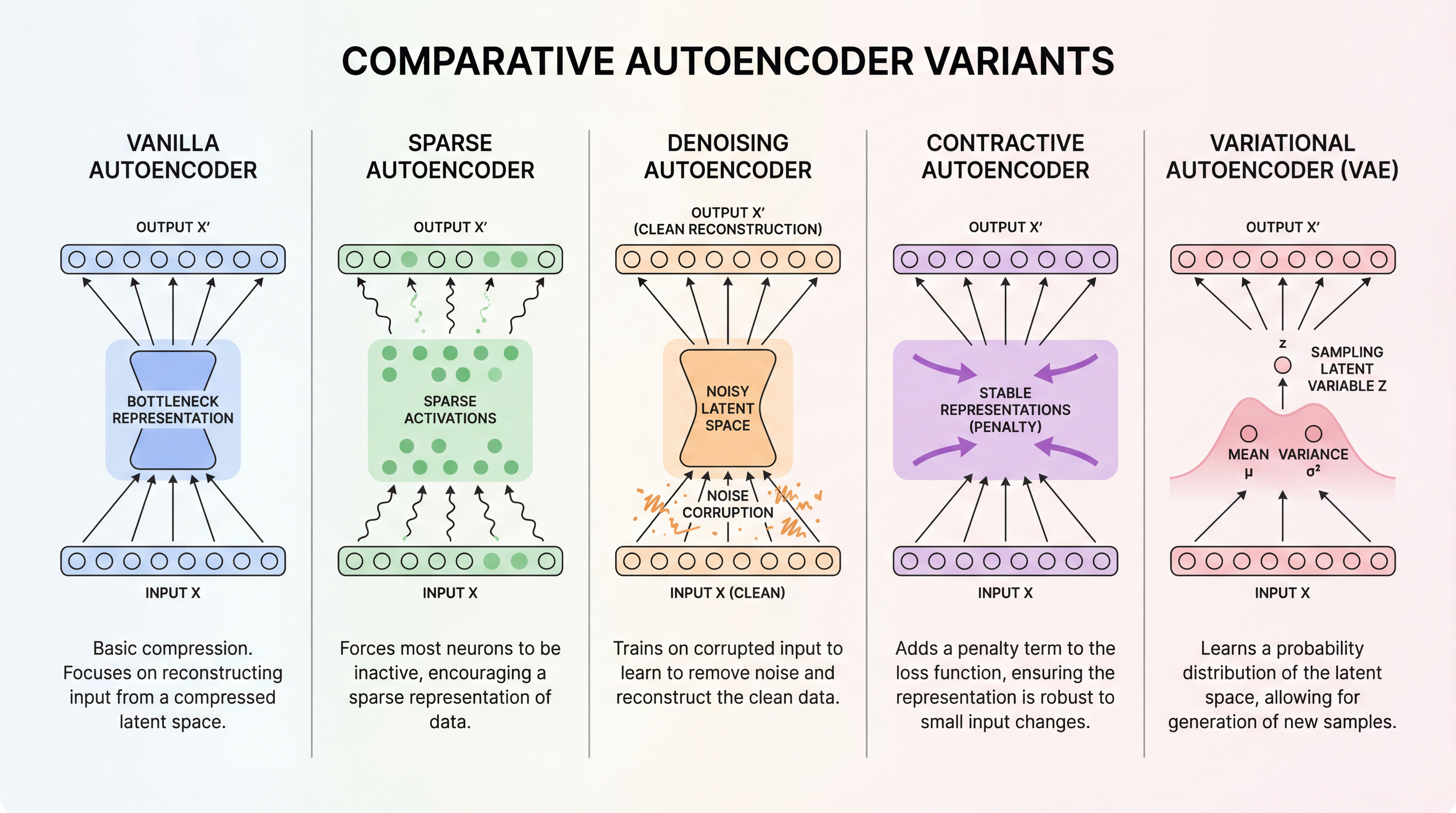
Part 5: Types of Autoencoders
There are several important variants. Each one adds a different constraint or regularization.
5.1 Vanilla Autoencoder
The simplest version: just encoder + decoder + MSE loss.
\[ \mathcal{L} = \|\mathbf{x} - g_\theta(f_\phi(\mathbf{x}))\|^2 \]
When to use: Basic feature learning, dimensionality reduction.
5.2 Sparse Autoencoder
Add a penalty to encourage most hidden units to be inactive:
\[ \mathcal{L} = \|\mathbf{x} - \hat{\mathbf{x}}\|^2 + \lambda \sum_j |h_j| \]
where \(h_j\) are the hidden activations and \(\lambda\) controls sparsity.
Intuition: Forces the network to use only a few features at a time, like how our brain might represent a face using only “has glasses”, “smiling”, “male”.
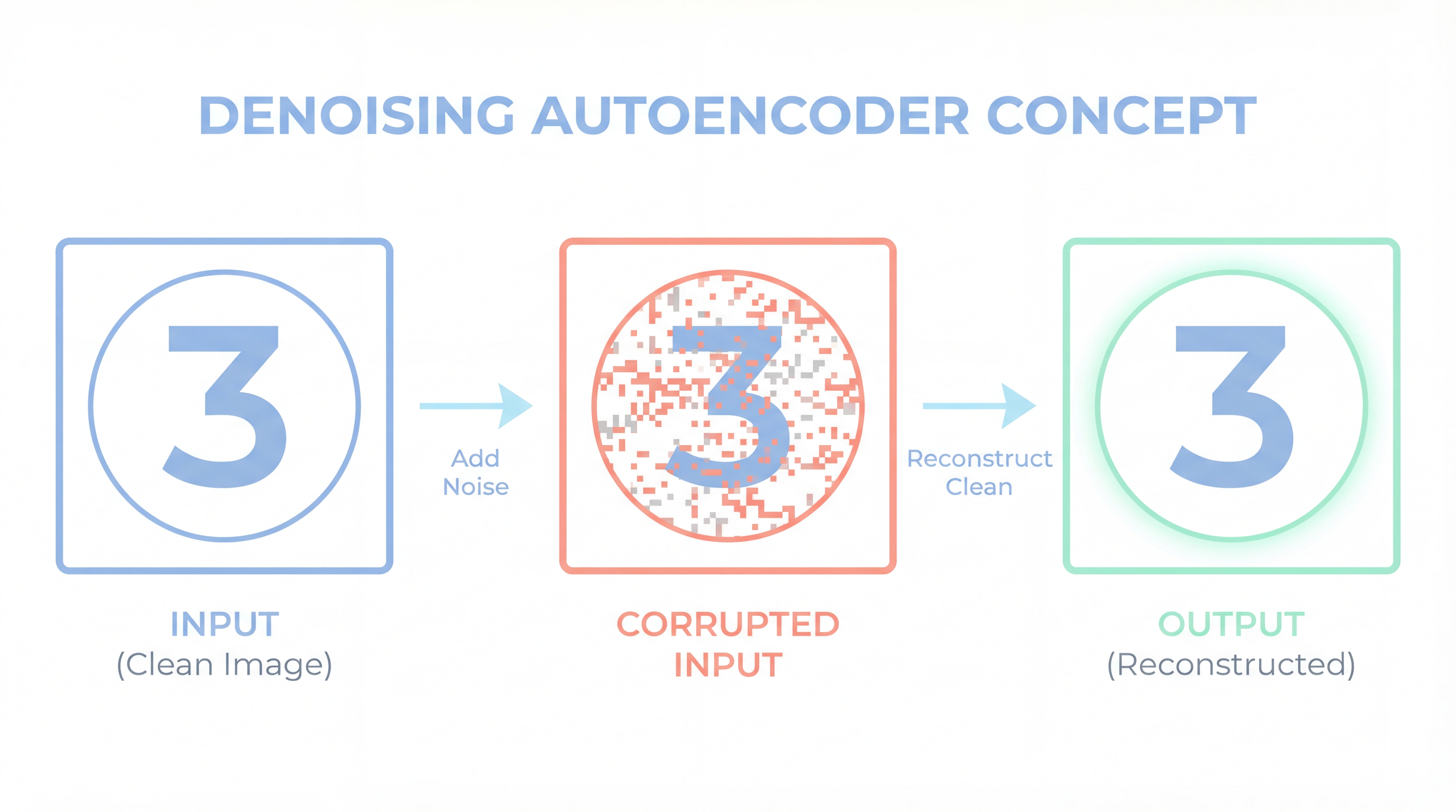
5.3 Denoising Autoencoder (DAE)
Corrupt the input first, then train to reconstruct the clean input:
\[ \mathcal{L} = \mathbb{E}_{\tilde{\mathbf{x}} \sim q(\tilde{\mathbf{x}} \mid \mathbf{x})} \left[ \|\mathbf{x} - g_\theta(f_\phi(\tilde{\mathbf{x}}))\|^2 \right] \]
Common corruptions:
- Add Gaussian noise: \(\tilde{\mathbf{x}} = \mathbf{x} + \epsilon\)
- Mask random pixels: \(\tilde{x}_i = 0\) with probability \(p\)
Intuition: Forces the network to learn robust features that can survive noise.
5.4 Contractive Autoencoder (CAE)
Penalize the encoder’s sensitivity to small input changes:
\[ \mathcal{L} = \|\mathbf{x} - \hat{\mathbf{x}}\|^2 + \lambda \|J_{f_\phi}(\mathbf{x})\|_F^2 \]
where \(J_{f_\phi}(\mathbf{x})\) is the Jacobian matrix of the encoder (how much each output changes for each input).
Intuition: Makes the latent representation stable—similar inputs should have similar codes.
5.5 Variational Autoencoder (VAE)
The encoder outputs a distribution instead of a point:
\[ q_\phi(\mathbf{z} \mid \mathbf{x}) = \mathcal{N}(\mathbf{z}; \boldsymbol{\mu}_\phi(\mathbf{x}), \text{diag}(\boldsymbol{\sigma}^2_\phi(\mathbf{x}))) \]
The loss has two parts:
\[ \mathcal{L}_{\text{VAE}} = \underbrace{\mathbb{E}_{q_\phi(\mathbf{z} \mid \mathbf{x})}[-\log p_\theta(\mathbf{x} \mid \mathbf{z})]}_{\text{Reconstruction}} + \underbrace{D_{\text{KL}}(q_\phi(\mathbf{z} \mid \mathbf{x}) \| p(\mathbf{z}))}_{\text{Regularization}} \]
Intuition: VAEs learn a smooth, continuous latent space where you can sample new data points!
Quick Reference Table
| Variant | Added Constraint | Main Use Case |
|---|---|---|
| Vanilla | Bottleneck only | Feature learning |
| Sparse | Sparsity penalty on activations | Interpretable features |
| Denoising | Corrupted input | Robustness, denoising |
| Contractive | Jacobian penalty | Stable representations |
| VAE | Probabilistic latent space | Generation, interpolation |
Part 6: PyTorch Implementation
Let us build a working autoencoder from scratch. We will use the sklearn digits dataset (8×8 grayscale digits) because:
- No download needed
- Fast to train on CPU
- Small enough to visualize the 2D latent space
6.1 Setup and Data Loading
# Load the digits dataset
digits = load_digits()

# Normalize pixels to [0, 1] range
X = (digits.images / 16.0).astype(np.float32)  # Original range is [0, 16]
y = digits.target.astype(np.int64)

# Flatten images: (N, 8, 8) -> (N, 64)
X_flat = X.reshape(len(X), -1)

# Split into train/test
X_train, X_test, y_train, y_test = train_test_split(
    X_flat, y, test_size=0.2, random_state=42, stratify=y
)

# Create PyTorch datasets
train_ds = TensorDataset(torch.tensor(X_train), torch.tensor(y_train))
test_ds = TensorDataset(torch.tensor(X_test), torch.tensor(y_test))

# Create data loaders
train_loader = DataLoader(train_ds, batch_size=128, shuffle=True)
test_loader = DataLoader(test_ds, batch_size=128, shuffle=False)

print(f"Training samples: {len(X_train)}")
print(f"Test samples: {len(X_test)}")
print(f"Input dimension: {X_flat.shape[1]} (8×8 = 64 pixels)")
print(f"Pixel range: [{X.min():.2f}, {X.max():.2f}]")
# Visualize some samples
fig, axes = plt.subplots(2, 6, figsize=(10, 4))
for ax, idx in zip(axes.ravel(), range(12)):
ax.imshow(X[idx], cmap="Blues", vmin=0, vmax=1)
ax.set_title(f"Label: {y[idx]}", fontsize=10)
ax.axis("off")
plt.suptitle("Sample Digits from the Dataset", fontsize=14, fontweight="bold", y=1.02)
plt.tight_layout()
plt.show()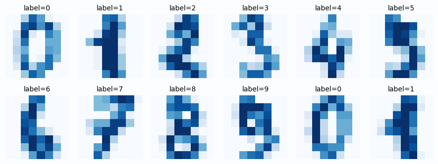
6.2 Define the Autoencoder Architecture
class Autoencoder(nn.Module):
    """
    A simple fully-connected autoencoder.

    Architecture:
    - Encoder: 64 -> 32 -> 16 -> 2 (bottleneck)
    - Decoder: 2 -> 16 -> 32 -> 64

    The 2D bottleneck allows us to visualize the latent space!
    """

    def __init__(self, input_dim=64, latent_dim=2):
        super().__init__()

        # Encoder: compress input to latent space
        self.encoder = nn.Sequential(
            nn.Linear(input_dim, 32),   # 64 -> 32
            nn.ReLU(),
            nn.Linear(32, 16),           # 32 -> 16
            nn.ReLU(),
            nn.Linear(16, latent_dim),   # 16 -> 2 (bottleneck!)
        )

        # Decoder: reconstruct from latent space
        self.decoder = nn.Sequential(
            nn.Linear(latent_dim, 16),   # 2 -> 16
            nn.ReLU(),
            nn.Linear(16, 32),           # 16 -> 32
            nn.ReLU(),
            nn.Linear(32, input_dim),    # 32 -> 64
            nn.Sigmoid(),                # Output in [0, 1] to match pixel range
        )

    def encode(self, x):
        """Map input to latent code."""
        return self.encoder(x)

    def decode(self, z):
        """Map latent code to reconstruction."""
        return self.decoder(z)

    def forward(self, x):
        """Full forward pass: encode then decode."""
        z = self.encode(x)
        x_hat = self.decode(z)
        return x_hat, z

# Create the model
model = Autoencoder(input_dim=64, latent_dim=2).to(device)

# Count parameters
total_params = sum(p.numel() for p in model.parameters())
print(f"Model architecture:\n{model}")
print(f"\nTotal parameters: {total_params:,}")
Why Sigmoid at the Output?
Our input pixels are in \([0, 1]\). The Sigmoid function ensures the reconstruction is also in \([0, 1]\), which makes the MSE loss well-behaved. For other data ranges, you might use different activations (or none).
6.3 Training Loop
# Loss function: Mean Squared Error
criterion = nn.MSELoss()

# Optimizer: Adam with default learning rate
optimizer = torch.optim.Adam(model.parameters(), lr=1e-3)

# Training settings
num_epochs = 100
history = {"train_loss": [], "test_loss": []}

print("Starting training...")
print("-" * 50)

for epoch in range(num_epochs):
    # === Training phase ===
    model.train()
    train_loss = 0.0

    for batch_x, _ in train_loader:  # We ignore labels (unsupervised!)
        batch_x = batch_x.to(device)

        # Forward pass
        x_hat, z = model(batch_x)
        loss = criterion(x_hat, batch_x)

        # Backward pass
        optimizer.zero_grad()
        loss.backward()
        optimizer.step()

        train_loss += loss.item() * batch_x.size(0)

    train_loss /= len(train_loader.dataset)
    history["train_loss"].append(train_loss)

    # === Evaluation phase ===
    model.eval()
    test_loss = 0.0

    with torch.no_grad():
        for batch_x, _ in test_loader:
            batch_x = batch_x.to(device)
            x_hat, z = model(batch_x)
            test_loss += criterion(x_hat, batch_x).item() * batch_x.size(0)

    test_loss /= len(test_loader.dataset)
    history["test_loss"].append(test_loss)

    # Print progress every 20 epochs
    if (epoch + 1) % 20 == 0:
        print(f"Epoch [{epoch+1:3d}/{num_epochs}]  Train Loss: {train_loss:.4f}  Test Loss: {test_loss:.4f}")

print("-" * 50)
print(f"Final Train Loss: {history['train_loss'][-1]:.4f}")
print(f"Final Test Loss:  {history['test_loss'][-1]:.4f}")
# Plot training curves
fig, ax = plt.subplots(figsize=(9, 5))
ax.plot(history["train_loss"], label="Train Loss", color="#6366f1", linewidth=2.5)
ax.plot(history["test_loss"], label="Test Loss", color="#10b981", linewidth=2.5, linestyle="--")
ax.scatter([len(history["train_loss"])-1], [history["train_loss"][-1]],
color="#6366f1", s=80, zorder=5)
ax.scatter([len(history["test_loss"])-1], [history["test_loss"][-1]],
color="#10b981", s=80, zorder=5)
ax.set_xlabel("Epoch", fontsize=12)
ax.set_ylabel("MSE Loss", fontsize=12)
ax.set_title("Autoencoder Training Curve", fontsize=14, fontweight="bold")
ax.legend(fontsize=11)
ax.grid(alpha=0.3)
ax.set_xlim(0, num_epochs)
plt.tight_layout()
plt.show()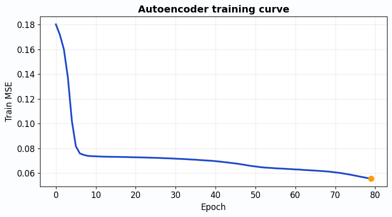
6.4 Visualize Reconstructions
# Get a batch of test images
model.eval()
test_batch_x, test_batch_y = next(iter(test_loader))
test_batch_x = test_batch_x.to(device)

with torch.no_grad():
    reconstructions, latent_codes = model(test_batch_x)

# Move to CPU for plotting
original = test_batch_x.cpu().numpy()
reconstructed = reconstructions.cpu().numpy()
labels = test_batch_y.numpy()

# Plot comparisons
n_samples = 8
fig, axes = plt.subplots(2, n_samples, figsize=(14, 4))

for i in range(n_samples):
    # Original
    axes[0, i].imshow(original[i].reshape(8, 8), cmap="Blues", vmin=0, vmax=1)
    axes[0, i].set_title(f"Label: {labels[i]}", fontsize=10)
    axes[0, i].axis("off")

    # Reconstruction
    axes[1, i].imshow(reconstructed[i].reshape(8, 8), cmap="Blues", vmin=0, vmax=1)
    axes[1, i].axis("off")

axes[0, 0].set_ylabel("Original", fontsize=12, rotation=0, labelpad=50, va="center")
axes[1, 0].set_ylabel("Reconstructed", fontsize=12, rotation=0, labelpad=50, va="center")

plt.suptitle("Original vs Reconstructed Digits (from 2D latent code)",
             fontsize=14, fontweight="bold", y=1.02)
plt.tight_layout()
plt.show()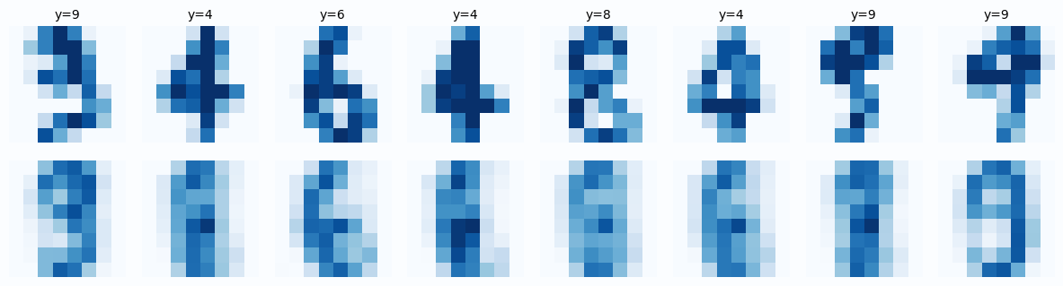
Observations
- The overall shape of each digit is preserved
- Some fine details are lost (the reconstruction is slightly blurry)
- This is expected! We compressed 64 dimensions into just 2
This is the fundamental compression vs quality tradeoff.
6.5 Visualize the Latent Space
This is the coolest part! Since our latent space is 2D, we can directly plot it.
# Collect all latent codes
all_z = []
all_y = []

model.eval()
with torch.no_grad():
    for batch_x, batch_y in test_loader:
        batch_x = batch_x.to(device)
        _, z = model(batch_x)
        all_z.append(z.cpu().numpy())
        all_y.append(batch_y.numpy())

all_z = np.concatenate(all_z, axis=0)
all_y = np.concatenate(all_y, axis=0)

# Create the plot
fig, ax = plt.subplots(figsize=(10, 8))

# Plot each digit class with a different color
scatter = ax.scatter(
    all_z[:, 0], all_z[:, 1],
    c=all_y,
    cmap="tab10",
    s=40,
    alpha=0.8,
    edgecolors="white",
    linewidths=0.5,
)

ax.set_xlabel("$z_1$ (First Latent Dimension)", fontsize=12)
ax.set_ylabel("$z_2$ (Second Latent Dimension)", fontsize=12)
ax.set_title("2D Latent Space Learned by the Autoencoder", fontsize=14, fontweight="bold")
ax.grid(alpha=0.2)

# Add colorbar with digit labels
cbar = plt.colorbar(scatter, ax=ax, ticks=range(10))
cbar.set_label("Digit Label", fontsize=11)
cbar.ax.set_yticklabels([str(i) for i in range(10)])

plt.tight_layout()
plt.show()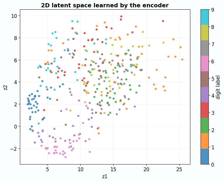
What Does This Plot Tell Us?
- Clustering: Digits of the same class cluster together (all 0s are near each other)
- Structure: Similar digits (like 4 and 9) are closer than dissimilar ones (like 0 and 1)
- Meaningful representation: The 2D code captures semantic information, even though we never used labels!
This is the power of autoencoders: they learn meaningful features through pure reconstruction.
6.6 Bonus: Generate New Digits by Sampling
Since we have a 2D latent space, we can pick any point and decode it to generate a digit.
# Create a grid of points in latent space
n_grid = 10
z1_range = np.linspace(all_z[:, 0].min() - 1, all_z[:, 0].max() + 1, n_grid)
z2_range = np.linspace(all_z[:, 1].min() - 1, all_z[:, 1].max() + 1, n_grid)

fig, axes = plt.subplots(n_grid, n_grid, figsize=(12, 12))

model.eval()
with torch.no_grad():
    for i, z2 in enumerate(reversed(z2_range)):  # Reverse so top = high z2
        for j, z1 in enumerate(z1_range):
            # Create latent code
            z = torch.tensor([[z1, z2]], dtype=torch.float32).to(device)

            # Decode
            x_hat = model.decode(z).cpu().numpy().reshape(8, 8)

            # Plot
            axes[i, j].imshow(x_hat, cmap="Blues", vmin=0, vmax=1)
            axes[i, j].axis("off")

plt.suptitle("Digits Generated by Decoding Points in Latent Space",
             fontsize=14, fontweight="bold", y=1.01)
plt.tight_layout()
plt.show()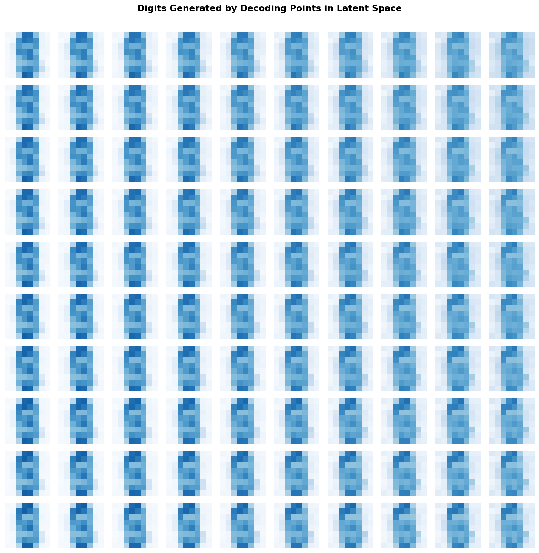
Part 7: Key Takeaways
Let us summarize everything we learned.
The Big Picture
- What: An autoencoder learns to reconstruct its input through a bottleneck
- Why: The bottleneck forces it to learn the essential structure of the data
- How: Minimize reconstruction error (MSE = Gaussian log-likelihood)
- Linear case: Equivalent to PCA
- Probabilistic view: Encoder infers latent cause, decoder models observations
- Variants: Sparse, denoising, contractive, variational (each adds a constraint)
The One Question to Remember
What is the smallest code that still lets me rebuild the input well?
If you understand this question, you understand autoencoders.
When to Use Autoencoders
| Use Case | Why Autoencoders Help |
|---|---|
| Dimensionality reduction | Learn a compact representation |
| Feature learning | Latent code captures meaningful structure |
| Anomaly detection | Normal data has low reconstruction error |
| Denoising | Train on noisy input, target clean output |
| Generative modeling | VAEs can sample new data |
| Pretraining | Initialize weights for supervised tasks |
Further Reading
This tutorial was inspired by the survey:
“Autoencoders” by Dor Bank, Noam Koenigstein, and Raja Giryes arXiv:2003.05991
For going deeper:
- VAEs: Kingma & Welling, “Auto-Encoding Variational Bayes” (2013)
- Denoising AEs: Vincent et al., “Extracting and Composing Robust Features” (2008)
- Contractive AEs: Rifai et al., “Contractive Auto-Encoders” (2011)
Feedback Welcome!
If you found this tutorial helpful or have suggestions for improvement, feel free to reach out. Happy learning!