Bayes’ Theorem: Intuition, NumPy, and Real-World Inference

A student-first Q&A guide to reasoning under uncertainty with visible plots and practical examples

Bayesian Thinking for Students

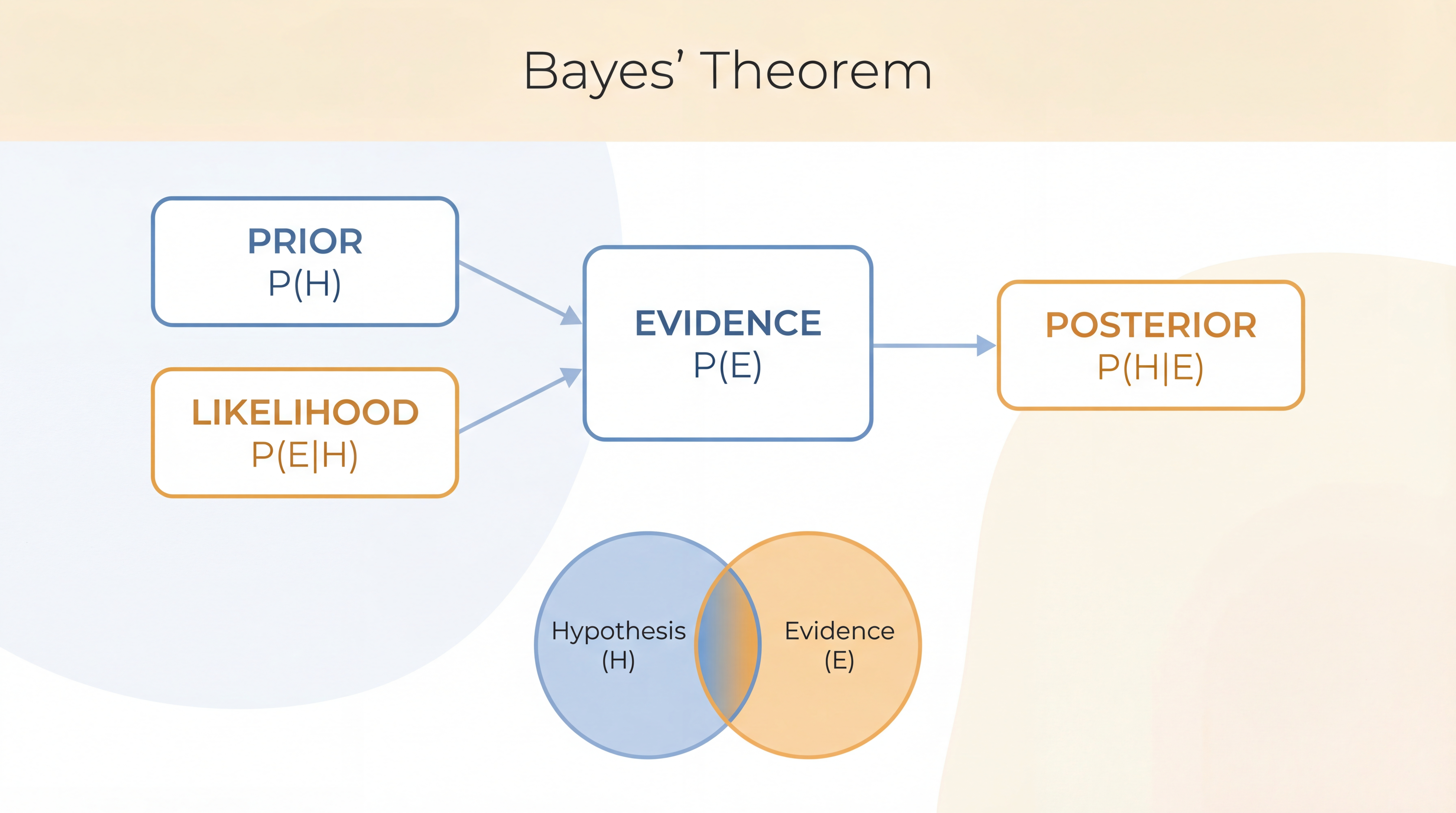
Bayes’ Theorem

Bayes’ theorem looks like a formula, but it is really a way of updating belief when new evidence arrives. This post is written to make that update feel intuitive, visual, and computationally concrete with NumPy.

This guide is designed to work in three ways:

• as a student-first explanation of conditional probability
• as a problem-solving tutorial with NumPy and visible plots
• as an interview-prep guide with a dropdown question after every topic

What You Will Build Intuition For

• Prior, likelihood, evidence, and posterior
• Why the base-rate fallacy feels so convincing
• How to turn Bayes’ theorem into NumPy code
• Why Bayes shows up in diagnosis, spam filtering, and machine learning

Student Friendly The math is introduced through intuition first, formula second.

Visible Plots Matplotlib figures are shown directly, while the plotting code is hidden in dropdowns.

NumPy Driven Every major calculation is written in a way you can reproduce and extend.

A light-theme Bayes’ theorem intuition graphic connecting prior, likelihood, evidence, posterior, and overlapping probability regions.

Learning Promise

By the end, you should be able to:

• read Bayes’ theorem in words instead of symbols only
• compute posteriors using counts and probabilities
• build NumPy-based Bayes calculations from scratch
• interpret why posterior belief can differ sharply from prior belief

This post is especially inspired by the visual, area-based intuition popularized by 3Blue1Brown and the machine-learning framing used by Machine Learning. Links are included in the reference section.

import numpy as np
import matplotlib.pyplot as plt

plt.style.use("default")
plt.rcParams["figure.figsize"] = (8, 5)
plt.rcParams["axes.spines.top"] = False
plt.rcParams["axes.spines.right"] = False
plt.rcParams["axes.grid"] = True
plt.rcParams["grid.alpha"] = 0.18

BLUE = "#4c78a8"
ORANGE = "#f28e2b"
GREEN = "#59a14f"
RED = "#e15759"
GRAY = "#bab0ac"
CREAM = "#fff6eb"

rng = np.random.default_rng(42)
print("NumPy version:", np.__version__)

NumPy version: 1.24.4

Part 1: The Core Question

Q1. What question does Bayes’ theorem actually answer?

Answer: Bayes’ theorem answers a very specific question:

If I observe some evidence, how should I update my belief about a hypothesis?

That is the heart of Bayesian reasoning. You start with a belief before seeing evidence, then revise it after seeing evidence.

The everyday structure looks like this:

• I had an initial belief.
• I saw a clue.
• I want to know how much that clue should change my belief.

This is why Bayes’ theorem appears in:

• medical testing
• spam filtering
• diagnosis
• search and recommendation
• machine learning classification

The theorem is not only about probability symbols. It is about belief revision under uncertainty.

That phrasing matters. Many students first meet Bayes’ theorem as a formula to memorize. That usually makes it feel harder than it really is. The deeper view is simpler:

• there is some hidden state you care about
• there is some observable signal you receive
• you want to connect the signal back to the hidden state

In other words, Bayes is useful whenever reality is partly hidden and all you get are clues.

That is why it appears in problems like:

• “Given this symptom, how likely is the disease?”
• “Given these words, how likely is spam?”
• “Given these sensor readings, how likely is a fault?”
• “Given this sequence of events, which explanation is now most plausible?”

Once you see Bayes that way, the formula stops being isolated math. It becomes a general reasoning pattern.

Interview Check: What is the central job of Bayes’ theorem in one sentence?

Its central job is to update the probability of a hypothesis after observing new evidence.

Q2. What do prior, likelihood, evidence, and posterior really mean?

Answer: These four words are the vocabulary of Bayes’ theorem.

Term	Meaning	Simple question
Prior	Belief before seeing the new evidence	What did I believe before the clue arrived?
Likelihood	How compatible the evidence is with the hypothesis	If the hypothesis were true, how likely is this clue?
Evidence	Overall probability of seeing the clue	How surprising is this clue overall?
Posterior	Updated belief after using the clue	What should I believe now?

A student-friendly way to remember this is:

• Prior = start
• Likelihood = fit of the clue
• Evidence = normalizing denominator
• Posterior = final updated belief

If that vocabulary feels abstract, think about a disease test:

• prior = disease prevalence before the test result
• likelihood = how likely a positive test is if a person truly has the disease
• evidence = how often positive tests happen overall
• posterior = probability the person truly has the disease after a positive result

One subtle but important point is that the likelihood is not a probability of the hypothesis. Students often mix this up.

• P(E | H) asks about the evidence under the hypothesis.
• P(H | E) asks about the hypothesis after seeing the evidence.

Those look similar on paper, but they answer different questions. Bayes’ theorem is the bridge between them.

Another useful way to think about these terms is as a story:

1. Prior: what you believed before the new clue.
2. Likelihood: how well the clue fits a given explanation.
3. Evidence: how common the clue is overall.
4. Posterior: what you believe after combining all of that.

That story structure makes Bayes much easier to apply in interviews and exams, because you can map almost every word problem onto it.

Interview Check: What is the difference between prior and posterior?

The prior is your belief before seeing the evidence, while the posterior is your updated belief after using the evidence.

Q3. What does conditional probability mean before Bayes even enters the picture?

Answer: Before Bayes’ theorem, you need one simpler idea:

conditional probability means we restrict attention to a smaller world where some condition is already known to be true.

If I ask for P(H | E), I am saying:

• ignore all cases where E did not happen
• focus only on the cases where E happened
• ask what fraction of that smaller group also satisfies H

That is why the vertical bar | is often read as “given that”.

Let us make that idea concrete with counts. Suppose we have a table of people, where:

• row 1 means the hypothesis is true
• row 2 means the hypothesis is false
• column 1 means the evidence is present
• column 2 means the evidence is absent

counts = np.array([
    [8, 2],    # hypothesis true
    [20, 170], # hypothesis false
])

total_cases = counts.sum()
evidence_cases = counts[:, 0].sum()
hypothesis_and_evidence = counts[0, 0]

p_h = counts[0].sum() / total_cases
p_e = evidence_cases / total_cases
p_h_given_e = hypothesis_and_evidence / evidence_cases

print("Total cases:", total_cases)
print("P(H):", round(p_h, 4))
print("P(E):", round(p_e, 4))
print("P(H | E):", round(p_h_given_e, 4))

Total cases: 200
P(H): 0.05
P(E): 0.14
P(H | E): 0.2857

The important move is this:

• for P(H), you divide by all cases
• for P(H | E), you divide only by the cases where evidence is present

That “change of denominator” is the entire intuition behind conditioning.

If you remember that, Bayes’ theorem becomes much easier because it is really about computing a conditional probability when it is hard to measure directly.

Interview Check: What changes when we move from P(H) to P(H | E)?

The reference group changes: instead of dividing by all cases, we divide only by the cases where the evidence is true.

Part 2: Reading the Formula Without Fear

Q4. What is Bayes’ theorem, and how should I read it in plain language?

Answer: The formula is:

\[ P(H \mid E) = \frac{P(E \mid H)\,P(H)}{P(E)} \]

Read it as:

The probability of the hypothesis given the evidence equals the probability of the evidence under the hypothesis, multiplied by the prior probability of the hypothesis, divided by the total probability of the evidence.

Or even more simply:

posterior = likelihood x prior / evidence

The most common mistake is to mix up these two quantities:

• P(H | E) = probability of the hypothesis after seeing the evidence
• P(E | H) = probability of seeing the evidence if the hypothesis were true

They are not the same thing.

Let’s compute a simple Bayes update with NumPy:

prior = 0.01
sensitivity = 0.99
false_positive_rate = 0.05

evidence = sensitivity * prior + false_positive_rate * (1 - prior)
posterior = sensitivity * prior / evidence

print(f"Prior probability: {prior:.4f}")
print(f"Evidence probability: {evidence:.4f}")
print(f"Posterior probability: {posterior:.4f}")

Prior probability: 0.0100
Evidence probability: 0.0594
Posterior probability: 0.1667

The evidence term is what keeps the result a valid probability. Without it, you would only have an unnormalized score.

There is also a very practical way to read the formula:

• start from the prior
• reward the hypothesis if the evidence fits it well
• then divide by how common the evidence is overall

That last step matters because evidence should count less if it is common everywhere. A clue that appears under almost every explanation is not very informative. A clue that strongly favors one explanation over others is much more informative.

Interview Check: Why is P(H|E) generally not equal to P(E|H)?

Because one asks how likely the hypothesis is after the evidence, while the other asks how likely the evidence is if the hypothesis were true. They answer different conditional questions.

Q5. Why is the denominator P(E) so important, and where does it come from?

Answer: The denominator is the probability of seeing the evidence at all. It is often called the evidence or the marginal probability of the evidence.

In many beginner problems, this is the part people do not know how to compute. The trick is:

break the evidence into all mutually exclusive ways it could happen, then add those pieces.

In the simple binary case:

\[ P(E) = P(E \mid H)P(H) + P(E \mid \neg H)P(\neg H) \]

This is just the law of total probability.

For the medical-testing example:

• evidence can come from a true positive
• or from a false positive

So the total probability of a positive test is the sum of those two routes.

prior = 0.01
not_prior = 1 - prior
sensitivity = 0.99
false_positive_rate = 0.05

positive_from_disease = sensitivity * prior
positive_from_healthy = false_positive_rate * not_prior
evidence = positive_from_disease + positive_from_healthy

print("Positive via true disease:", round(positive_from_disease, 5))
print("Positive via healthy group:", round(positive_from_healthy, 5))
print("Total evidence P(positive):", round(evidence, 5))

Positive via true disease: 0.0099
Positive via healthy group: 0.0495
Total evidence P(positive): 0.0594

This section is worth slowing down for, because it explains why Bayes is not a magic trick. The denominator is not mysterious. It is just the total size of the evidence pool.

If you think in counts, it becomes even clearer:

• numerator = the part of the evidence pool that supports the hypothesis
• denominator = the whole evidence pool

That is exactly why the posterior is a fraction of one region inside another.

Interview Check: In a binary Bayes problem, what are the two most common pieces used to build P(E)?

They are the evidence coming from the hypothesis being true and the evidence coming from the hypothesis being false.

Q6. Why do counts and frequencies often feel easier than symbols?

Answer: Human intuition usually handles counts better than abstract percentages.

Suppose a disease has:

• prevalence = 1%
• sensitivity = 99%
• specificity = 95%

Instead of thinking in abstract probabilities, imagine 10,000 people:

• about 100 truly have the disease
• about 9,900 do not
• about 99 true positives appear
• about 495 false positives appear

Now the important question becomes:

Out of all positive tests, how many are truly sick?

That is easier to reason about than the formula alone.

population = 10_000
prevalence = 0.01
sensitivity = 0.99
specificity = 0.95

disease = int(population * prevalence)
healthy = population - disease

true_positive = int(round(sensitivity * disease))
false_negative = disease - true_positive
true_negative = int(round(specificity * healthy))
false_positive = healthy - true_negative

posterior_positive = true_positive / (true_positive + false_positive)

print("Disease cases:", disease)
print("Healthy cases:", healthy)
print("True positives:", true_positive)
print("False positives:", false_positive)
print("Posterior P(disease | positive):", round(posterior_positive, 4))

Disease cases: 100
Healthy cases: 9900
True positives: 99
False positives: 495
Posterior P(disease | positive): 0.1667

This is exactly the kind of perspective emphasized by visual explanations of Bayes: not “memorize the fraction,” but “see the fraction as a part of a whole.”

This is also why frequency language is powerful in teaching:

• “99 out of 100 sick people test positive”
• “495 healthy people still test positive”
• “So among all positive tests, only 99 are true positives”

That feels more human than a stack of symbols.

In interviews, if you get stuck on symbolic Bayes, converting the problem into an imaginary population like 1,000 or 10,000 often unlocks the answer immediately.

Interview Check: Why do frequency-based explanations often help students more than symbolic ones?

Because it is easier to picture actual counts like 99 true positives out of 594 positive tests than to reason purely with abstract symbols and conditional probabilities.

Q7. Can I build an area intuition instead of memorizing the formula?

Answer: Yes. This is one of the most helpful ways to think about Bayes’ theorem.

Imagine the full set of possibilities as a rectangle of area 1.

• the part where the hypothesis is true has area P(H)
• the part where the evidence is true has area P(E)
• the overlapping region has area P(H ∩ E)

Then:

\[ P(H \mid E) = \frac{P(H \cap E)}{P(E)} \]

That means:

once the evidence is known, we only look inside the evidence region, and then ask what fraction of that region belongs to the hypothesis.

This is deeply important because it turns Bayes into a geometric idea:

• evidence restricts the sample space
• the posterior is a proportion inside that restricted space

That is why the theorem feels so natural in the 3Blue1Brown explanation. It is not just algebra. It is a picture of how the world gets narrowed after a clue arrives.

The area view also explains an important sanity check:

• if the evidence is equally common whether H is true or false, the posterior should stay close to the prior
• if the evidence is much more common under H, the posterior should rise
• if the evidence is much less common under H, the posterior should fall

So even before calculation, Bayes gives you a directional intuition.

Interview Check: In the area interpretation, what does the denominator P(E) represent?

It represents the whole restricted evidence region inside which we measure the share belonging to the hypothesis.

Part 3: Medical Testing, Base Rates, and Visual Intuition

Q8. What are sensitivity and specificity, and why are they different?

Answer: These are two of the most important terms in medical-testing problems.

Sensitivity tells you how well a test catches people who really have the disease.

\[ \text{Sensitivity} = P(\text{positive} \mid \text{disease}) \]

So sensitivity answers:

if a person is truly sick, how likely is the test to come back positive?

Specificity tells you how well a test correctly clears people who do not have the disease.

\[ \text{Specificity} = P(\text{negative} \mid \text{healthy}) \]

So specificity answers:

if a person is truly healthy, how likely is the test to come back negative?

Students often confuse them because both measure “accuracy” in some sense, but they measure accuracy on different groups:

• sensitivity focuses on the sick group
• specificity focuses on the healthy group

Their complements are just as important:

• false negative rate = 1 - sensitivity
• false positive rate = 1 - specificity

Here is a tiny count-based example.

sick_people = 100
healthy_people = 100
sensitivity = 0.90
specificity = 0.95

true_positives = int(sick_people * sensitivity)
false_negatives = sick_people - true_positives
true_negatives = int(healthy_people * specificity)
false_positives = healthy_people - true_negatives

print("True positives:", true_positives)
print("False negatives:", false_negatives)
print("True negatives:", true_negatives)
print("False positives:", false_positives)

True positives: 90
False negatives: 10
True negatives: 95
False positives: 5

With these numbers:

• out of 100 sick people, 90 test positive
• out of 100 healthy people, 95 test negative

That is all sensitivity and specificity mean at the most practical level.

Interview Check: What is the difference between sensitivity and specificity?

Sensitivity measures how often truly sick people test positive, while specificity measures how often truly healthy people test negative.

Q9. Why does a positive medical test not automatically mean the disease is likely?

Answer: Because the base rate matters.

If the disease is rare, even a good test can generate many false positives simply because the healthy group is much larger than the sick group.

With the same numbers as above:

• disease prevalence = 1%
• sensitivity = 99%
• specificity = 95%

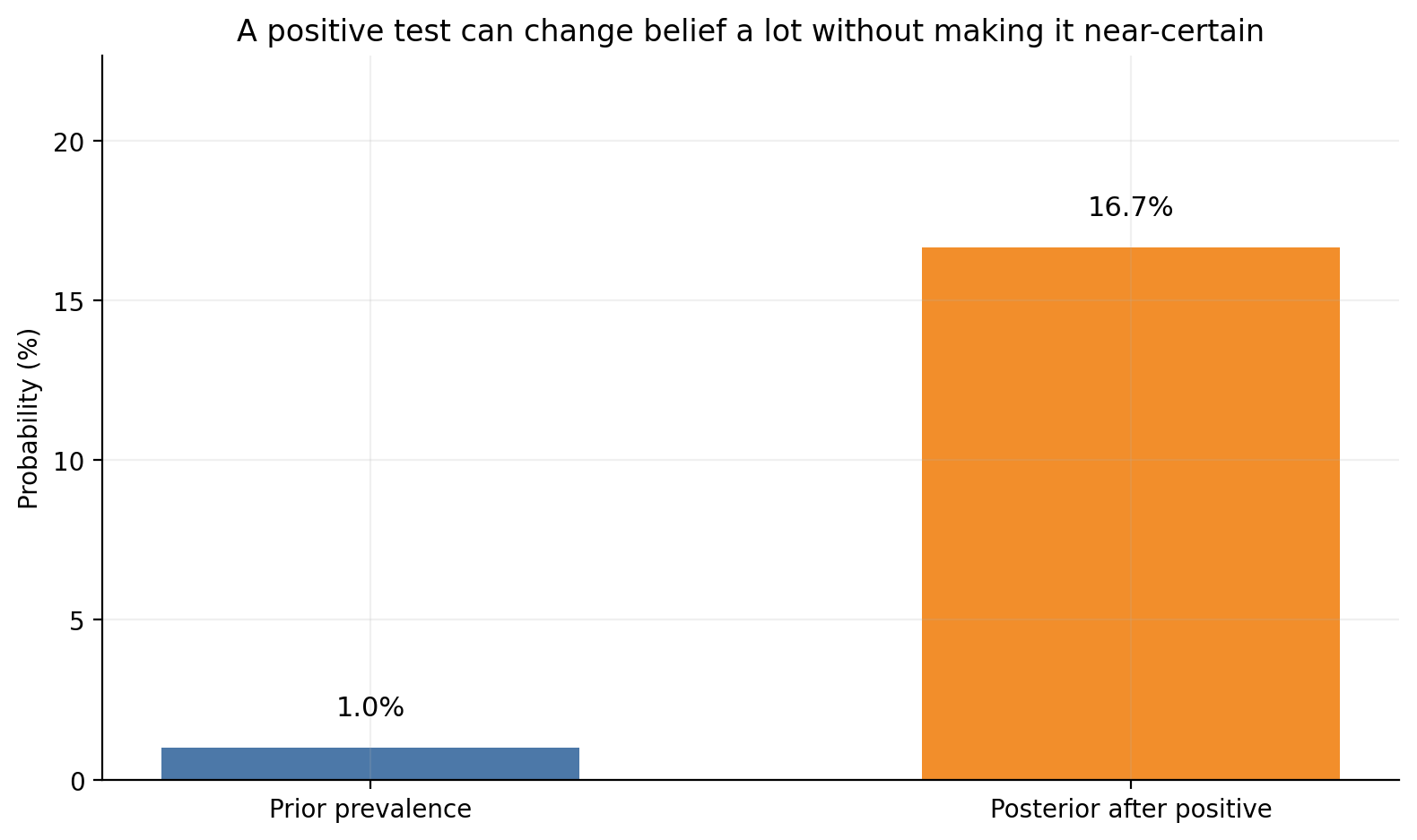
The prior is only 1%, but the posterior after a positive test is only around 16.7%, not 99%.

That feels surprising because people often confuse:

• test accuracy
• posterior probability

Those are not the same quantity.

prior = 0.01
sensitivity = 0.99
specificity = 0.95
posterior_positive = sensitivity * prior / (
    sensitivity * prior + (1 - specificity) * (1 - prior)
)

print(f"Prior prevalence: {prior:.2%}")
print(f"Posterior after a positive test: {posterior_positive:.2%}")

Prior prevalence: 1.00%
Posterior after a positive test: 16.67%

Show Matplotlib code for this figure

prior_pct = prior * 100
posterior_pct = posterior_positive * 100

fig, ax = plt.subplots(figsize=(8, 4.8))
bars = ax.bar(
    ["Prior prevalence", "Posterior after positive"],
    [prior_pct, posterior_pct],
    color=[BLUE, ORANGE],
    width=0.55
)

for bar, value in zip(bars, [prior_pct, posterior_pct]):
    ax.text(bar.get_x() + bar.get_width()/2, value + 1, f"{value:.1f}%", ha="center", fontsize=11)

ax.set_ylabel("Probability (%)")
ax.set_ylim(0, max(22, posterior_pct + 6))
ax.set_title("A positive test can change belief a lot without making it near-certain")
plt.tight_layout()
plt.show()

Interview Check: What is the base-rate fallacy in this context?

It is the mistake of focusing on the test result or test accuracy while ignoring how rare the disease was to begin with.

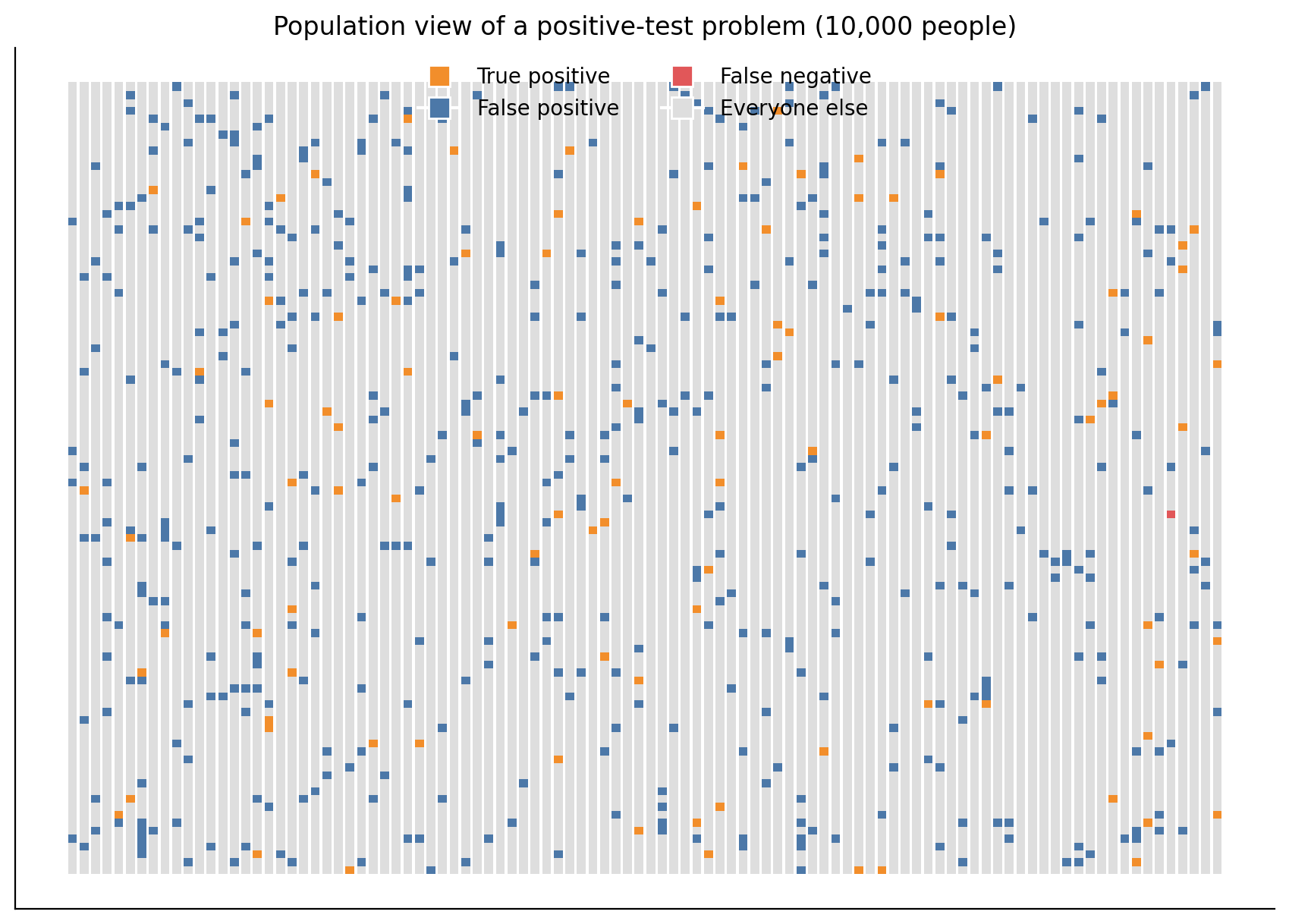
Q10. Can I make the same example feel visual using a population plot?

Answer: Yes. A population plot makes Bayes feel concrete.

Here we simulate 10,000 people and color-code:

• true positives
• false positives
• everyone else

The key insight is that even a relatively small false-positive rate can create many false positives when the healthy population is huge.

Show Matplotlib code for this figure

population = 10_000
labels = np.array(["Other"] * population, dtype=object)
labels[:true_positive] = "True positive"
labels[true_positive:true_positive + false_positive] = "False positive"
labels[true_positive + false_positive:true_positive + false_positive + false_negative] = "False negative"
rng = np.random.default_rng(7)
rng.shuffle(labels)

x = np.tile(np.arange(100), 100)
y = np.repeat(np.arange(100), 100)

colors = np.where(
    labels == "True positive", ORANGE,
    np.where(labels == "False positive", BLUE,
             np.where(labels == "False negative", RED, "#dedede"))
)

fig, ax = plt.subplots(figsize=(8.6, 6.2))
ax.scatter(x, y, c=colors, s=18, marker="s", linewidths=0)
ax.set_xticks([])
ax.set_yticks([])
ax.set_title("Population view of a positive-test problem (10,000 people)")

from matplotlib.lines import Line2D
legend_elements = [
    Line2D([0], [0], marker='s', color='w', label='True positive', markerfacecolor=ORANGE, markersize=10),
    Line2D([0], [0], marker='s', color='w', label='False positive', markerfacecolor=BLUE, markersize=10),
    Line2D([0], [0], marker='s', color='w', label='False negative', markerfacecolor=RED, markersize=10),
    Line2D([0], [0], marker='s', color='w', label='Everyone else', markerfacecolor='#dedede', markersize=10),
]
ax.legend(handles=legend_elements, loc="upper center", ncol=2, frameon=False)
plt.tight_layout()
plt.show()

Interview Check: Why can there be many false positives even when specificity is high?

Because the healthy group can be much larger than the sick group, so a small false-positive rate applied to a huge group still creates many false positives.

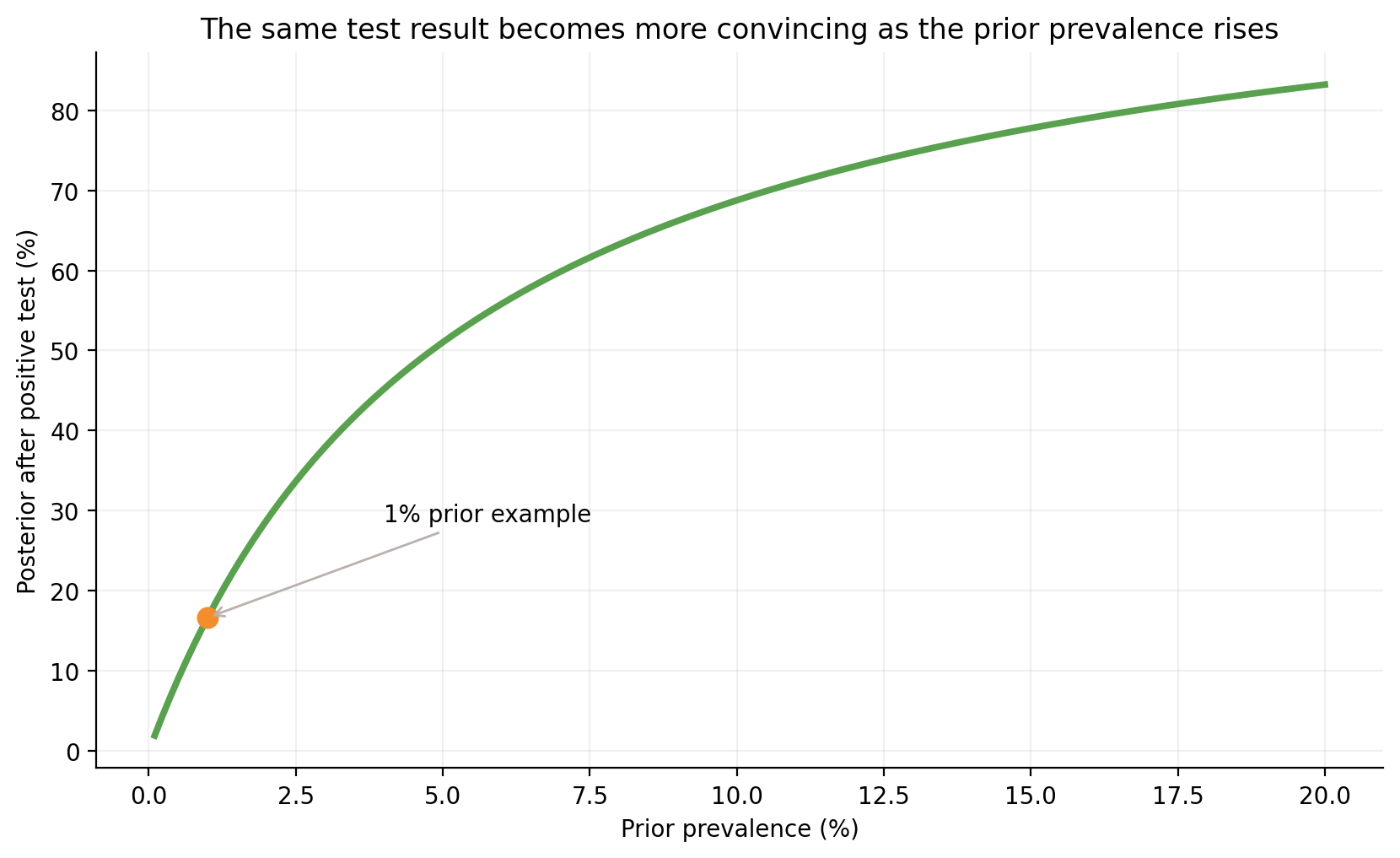
Q11. How does the posterior change as the prior prevalence changes?

Answer: This is one of the most important Bayes insights:

The same evidence can mean very different things when the prior changes.

For a fixed medical test:

• if prevalence is tiny, the posterior after a positive result may still be modest
• if prevalence is larger, the same positive result becomes much more convincing

Let’s sweep the prior prevalence from very small to moderately large values and compute the posterior after a positive test.

priors = np.linspace(0.001, 0.20, 300)
posterior_curve = sensitivity * priors / (
    sensitivity * priors + (1 - specificity) * (1 - priors)
)

print("Posterior at 1% prevalence:", round(float(posterior_curve[np.argmin(np.abs(priors - 0.01))]), 4))
print("Posterior at 10% prevalence:", round(float(posterior_curve[np.argmin(np.abs(priors - 0.10))]), 4))

Posterior at 1% prevalence: 0.1711
Posterior at 10% prevalence: 0.6879

Show Matplotlib code for this figure

fig, ax = plt.subplots(figsize=(8.4, 5.2))
ax.plot(priors * 100, posterior_curve * 100, color=GREEN, linewidth=2.8)
ax.scatter([1], [posterior_positive * 100], color=ORANGE, s=70, zorder=3)
ax.annotate("1% prior example", (1, posterior_positive * 100), xytext=(4, posterior_positive * 100 + 12),
            arrowprops=dict(arrowstyle="->", color=GRAY), fontsize=10)
ax.set_xlabel("Prior prevalence (%)")
ax.set_ylabel("Posterior after positive test (%)")
ax.set_title("The same test result becomes more convincing as the prior prevalence rises")
plt.tight_layout()
plt.show()

Interview Check: Why does the same positive test result lead to different posteriors under different priors?

Because Bayes’ theorem combines the evidence with the prior, so the starting belief changes how strongly the same evidence updates the final belief.

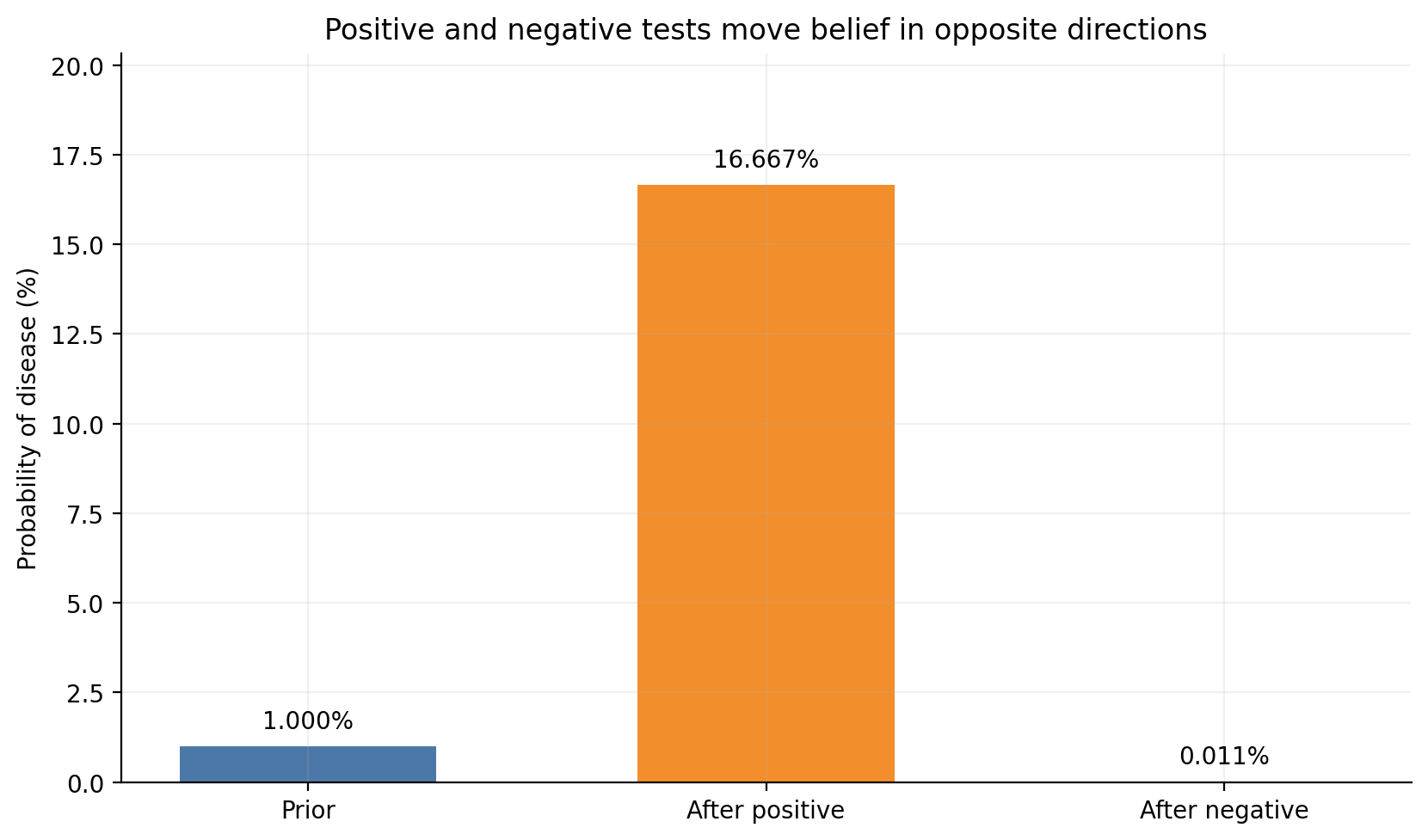
Q12. What happens after a negative test result, and why is that also a Bayes update?

Answer: Bayes’ theorem does not only work for positive evidence. A negative result is also evidence.

For the same test:

• P(negative | disease) = 1 - sensitivity
• P(negative | healthy) = specificity

So the posterior after a negative result is:

\[ P(\text{disease} \mid \text{negative}) = \frac{P(\text{negative} \mid \text{disease})P(\text{disease})}{P(\text{negative})} \]

Let us compute both updates side by side.

prior = 0.01
sensitivity = 0.99
specificity = 0.95

posterior_positive = sensitivity * prior / (
    sensitivity * prior + (1 - specificity) * (1 - prior)
)

posterior_negative = (1 - sensitivity) * prior / (
    (1 - sensitivity) * prior + specificity * (1 - prior)
)

print(f"P(disease): {prior:.4%}")
print(f"P(disease | positive): {posterior_positive:.4%}")
print(f"P(disease | negative): {posterior_negative:.4%}")

P(disease): 1.0000%
P(disease | positive): 16.6667%
P(disease | negative): 0.0106%

The positive result raises the belief sharply, while the negative result pushes it down to a tiny value. That makes intuitive sense:

• a positive test is evidence for disease
• a negative test is evidence against disease

But the strength of each update depends on the test characteristics. If sensitivity were poor, a negative result would not be very reassuring. If specificity were poor, a positive result would not be very convincing.

Show Matplotlib code for this figure

values = np.array([prior * 100, posterior_positive * 100, posterior_negative * 100])
labels = ["Prior", "After positive", "After negative"]

fig, ax = plt.subplots(figsize=(8.4, 5.0))
bars = ax.bar(labels, values, color=[BLUE, ORANGE, GREEN], width=0.56)

for bar, value in zip(bars, values):
    ax.text(
        bar.get_x() + bar.get_width() / 2,
        value + max(values) * 0.03,
        f"{value:.3f}%",
        ha="center",
        fontsize=10
    )

ax.set_ylabel("Probability of disease (%)")
ax.set_ylim(0, max(values) * 1.22)
ax.set_title("Positive and negative tests move belief in opposite directions")
plt.tight_layout()
plt.show()

Interview Check: Why can a negative result be much more reassuring than a positive result is convincing?

Because the update strength depends on sensitivity, specificity, and the base rate, and those may make negative evidence much stronger than positive evidence in a given problem.

Q13. How do likelihood ratios summarize the strength of evidence?

Answer: Likelihood ratios compress a Bayes update into a single “evidence strength” number.

For a medical test:

• positive likelihood ratio: LR+ = sensitivity / false_positive_rate
• negative likelihood ratio: LR- = false_negative_rate / specificity

These tell you how much the evidence shifts the odds.

• LR+ > 1 supports the hypothesis
• LR- < 1 supports the opposite
• the farther away from 1, the stronger the update

prior = 0.01
sensitivity = 0.99
specificity = 0.95

false_positive_rate = 1 - specificity
false_negative_rate = 1 - sensitivity

lr_positive = sensitivity / false_positive_rate
lr_negative = false_negative_rate / specificity

prior_odds = prior / (1 - prior)
posterior_odds_positive = prior_odds * lr_positive
posterior_from_odds = posterior_odds_positive / (1 + posterior_odds_positive)

print("LR+:", round(lr_positive, 4))
print("LR-:", round(lr_negative, 4))
print("Posterior via odds after positive:", round(posterior_from_odds, 4))

LR+: 19.8
LR-: 0.0105
Posterior via odds after positive: 0.1667

This is a slightly more advanced way to think, but it is extremely useful:

• Bayes in probability form updates probabilities
• Bayes in odds form updates odds

The odds form is often easier in diagnostics and decision-making because the evidence multiplier is explicit.

Interview Check: What does an LR+ far larger than 1 mean?

It means a positive result is much more likely when the hypothesis is true than when it is false, so the evidence strongly supports the hypothesis.

Part 4: Updating Beliefs with NumPy

Q14. How can I write Bayes’ theorem for multiple hypotheses using NumPy?

Answer: Bayes is not limited to one hypothesis versus not-hypothesis. You can update belief across many competing explanations at once.

Suppose you have three boxes:

• Box A
• Box B
• Box C

You start with prior probabilities for the boxes, then observe evidence such as drawing a red ball. Each box gives a different likelihood for seeing red.

priors = np.array([0.50, 0.30, 0.20])
likelihood_red = np.array([0.10, 0.70, 0.40])

unnormalized = priors * likelihood_red
posterior = unnormalized / unnormalized.sum()

print("Priors:", priors)
print("Likelihood of red under each box:", likelihood_red)
print("Posterior after observing red:", posterior.round(4))
print("Posterior sums to:", posterior.sum())

Priors: [0.5 0.3 0.2]
Likelihood of red under each box: [0.1 0.7 0.4]
Posterior after observing red: [0.1471 0.6176 0.2353]
Posterior sums to: 1.0

This is the vector form of Bayes:

1. multiply prior by likelihood
2. normalize by dividing through the total

That same pattern appears in hidden-state models, classification, sensor fusion, and probabilistic filtering.

Interview Check: Why do we divide by unnormalized.sum() in the multi-hypothesis case?

Because the raw scores must be normalized so that the posterior probabilities sum to 1.

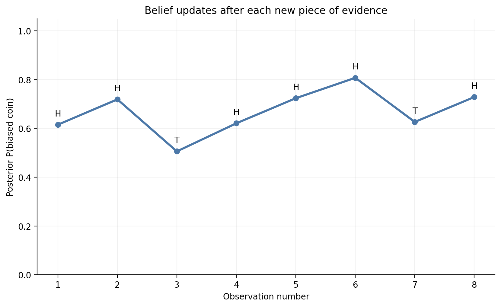
Q15. How do repeated pieces of evidence update a belief over time?

Answer: Bayes is not only for one update. It is naturally sequential.

Imagine two competing hypotheses:

• H_fair: the coin is fair, so P(H) = 0.5
• H_biased: the coin is biased toward heads, so P(H) = 0.8

Now suppose we observe a sequence of coin tosses:

H, H, T, H, H, H, T, H

After each toss, we update the posterior belief in the biased-coin hypothesis.

sequence = np.array(list("HHTHHHTH"))
prior_hyp = np.array([0.5, 0.5])   # fair, biased
p_heads = np.array([0.5, 0.8])
p_tails = 1 - p_heads

posteriors_biased = []
current = prior_hyp.copy()

for outcome in sequence:
    likelihood = p_heads if outcome == "H" else p_tails
    current = current * likelihood
    current = current / current.sum()
    posteriors_biased.append(current[1])

print("Posterior of biased hypothesis after final toss:", round(posteriors_biased[-1], 4))

Posterior of biased hypothesis after final toss: 0.7286

Show Matplotlib code for this figure

steps = np.arange(1, len(sequence) + 1)

fig, ax = plt.subplots(figsize=(8.4, 5.2))
ax.plot(steps, posteriors_biased, marker="o", color=BLUE, linewidth=2.5)
for i, outcome in enumerate(sequence):
    ax.text(steps[i], posteriors_biased[i] + 0.035, outcome, ha="center", fontsize=10)

ax.set_ylim(0, 1.05)
ax.set_xticks(steps)
ax.set_xlabel("Observation number")
ax.set_ylabel("Posterior P(biased coin)")
ax.set_title("Belief updates after each new piece of evidence")
plt.tight_layout()
plt.show()

This is one of the deepest ideas in Bayesian reasoning:

today’s posterior becomes tomorrow’s prior.

Interview Check: What does it mean to say that today’s posterior becomes tomorrow’s prior?

It means Bayesian updating can be repeated: after one observation updates your belief, that updated belief becomes the starting point for the next observation.

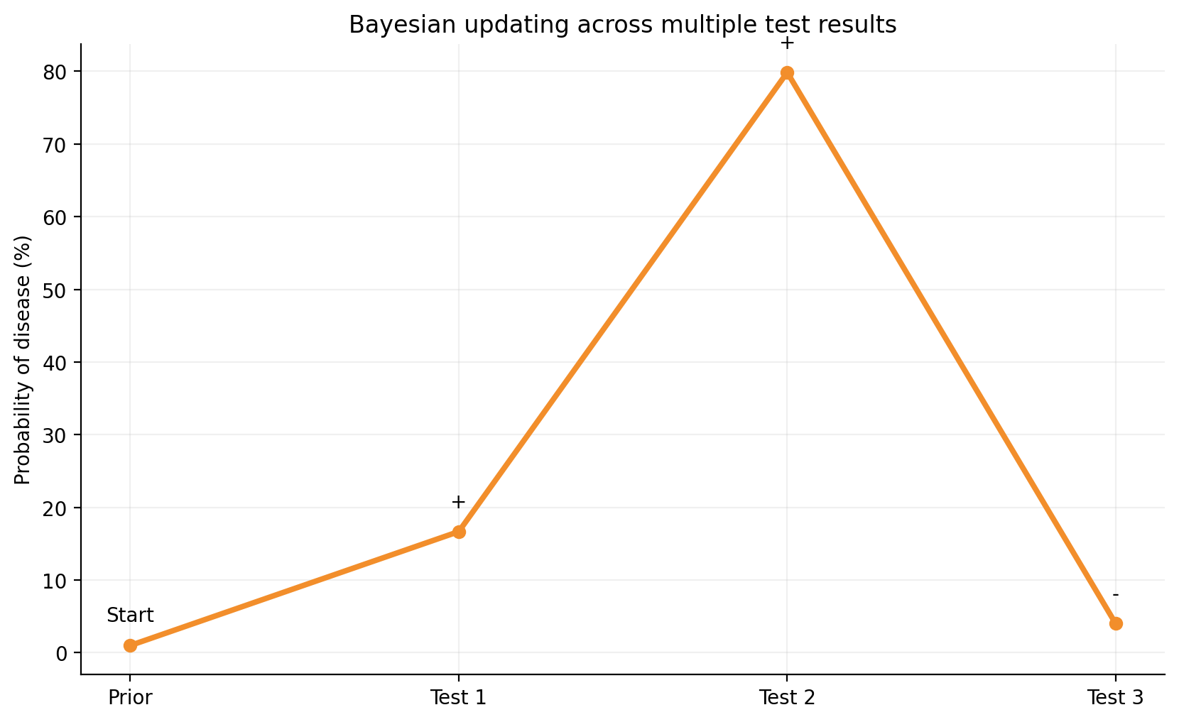
Q16. How do multiple test results update the same belief step by step?

Answer: The medical-testing example becomes much more realistic when you update repeatedly.

Suppose:

• disease prevalence starts at 1%
• you observe three test outcomes in sequence
• the outcomes are positive, positive, negative

After each observation, you use the previous posterior as the new prior.

def update_disease_probability(current_prior: float, result: str, sensitivity: float, specificity: float) -> float:
    if result == "positive":
        numerator = sensitivity * current_prior
        denominator = sensitivity * current_prior + (1 - specificity) * (1 - current_prior)
    else:
        numerator = (1 - sensitivity) * current_prior
        denominator = (1 - sensitivity) * current_prior + specificity * (1 - current_prior)
    return numerator / denominator

test_results = ["positive", "positive", "negative"]
current = 0.01
history = [current]

for result in test_results:
    current = update_disease_probability(current, result, sensitivity=0.99, specificity=0.95)
    history.append(current)

print("Posterior history:", np.round(history, 6))

Posterior history: [0.01     0.166667 0.798387 0.040016]

This is a powerful lesson:

• one result updates the belief
• the next result updates the already-updated belief
• the order and type of evidence both matter

Show Matplotlib code for this figure

steps = np.arange(len(history))
labels = ["Start", "+", "+", "-"]

fig, ax = plt.subplots(figsize=(8.4, 5.2))
ax.plot(steps, np.array(history) * 100, marker="o", color=ORANGE, linewidth=2.8)

for x_pos, y_pos, label in zip(steps, np.array(history) * 100, labels):
    ax.text(x_pos, y_pos + max(np.array(history) * 100) * 0.04 + 0.1, label, ha="center", fontsize=10)

ax.set_xticks(steps)
ax.set_xticklabels(["Prior", "Test 1", "Test 2", "Test 3"])
ax.set_ylabel("Probability of disease (%)")
ax.set_title("Bayesian updating across multiple test results")
plt.tight_layout()
plt.show()

Interview Check: Why is sequential Bayes especially natural for repeated measurements or tests?

Because each new result can be incorporated by treating the current posterior as the next prior, so evidence accumulates step by step.

Q17. Why do machine-learning implementations often use log probabilities instead of multiplying many tiny numbers directly?

Answer: Because direct multiplication of many small probabilities can underflow numerically.

In theory, multiplying likelihoods is fine. In practice, if you multiply hundreds of tiny numbers, a computer may store the result as 0.0.

That is why many implementations work with:

\[ \log(a b c) = \log a + \log b + \log c \]

This converts unstable products into stable sums.

likelihood_terms = np.full(400, 0.01)
direct_product = np.prod(likelihood_terms)
log_score = np.sum(np.log(likelihood_terms))

candidate_log_scores = np.array([log_score, log_score - 4.0, log_score - 8.0])
stable_scores = np.exp(candidate_log_scores - candidate_log_scores.max())
stable_posterior = stable_scores / stable_scores.sum()

print("Direct product:", direct_product)
print("Log score:", round(float(log_score), 3))
print("Stable posterior from log scores:", stable_posterior.round(4))

Direct product: 0.0
Log score: -1842.068
Stable posterior from log scores: [9.817e-01 1.800e-02 3.000e-04]

This is the same reason the Naive Bayes example later uses log probabilities before converting back to normalized scores.

For students, this is a nice bridge from probability to real software engineering:

• the math says multiply probabilities
• the implementation says sum log-probabilities
• both represent the same ranking logic

Interview Check: Why are log probabilities useful in Bayes-based machine-learning code?

They avoid numerical underflow and turn large products of tiny probabilities into manageable sums.

Part 5: Bayes in Machine Learning

Q18. Why does Bayes’ theorem matter in machine learning?

Answer: Bayes matters because many ML tasks are really about comparing competing explanations for observed data.

In classification, the structure is:

\[ P(\text{class} \mid \text{features}) \propto P(\text{features} \mid \text{class}) P(\text{class}) \]

That is exactly the Bayes pattern:

• prior over classes
• likelihood of features under each class
• posterior over classes after seeing the features

The classic example is Naive Bayes, which assumes feature independence given the class.

Consider a tiny spam-filtering example with two words: "free" and "meeting".

classes = np.array(["spam", "ham"])
priors = np.array([0.4, 0.6])

# Likelihood table: rows are classes, columns are words [free, meeting]
likelihood = np.array([
    [0.7, 0.1],  # spam
    [0.1, 0.6],  # ham
])

observed_words = np.array([1, 0])  # email contains "free" but not "meeting"

log_scores = np.log(priors) + np.sum(
    observed_words * np.log(likelihood) +
    (1 - observed_words) * np.log(1 - likelihood),
    axis=1
)

scores = np.exp(log_scores - log_scores.max())
posterior = scores / scores.sum()

print("Classes:", classes)
print("Posterior probabilities:", posterior.round(4))
print("Predicted class:", classes[np.argmax(posterior)])

Classes: ['spam' 'ham']
Posterior probabilities: [0.913 0.087]
Predicted class: spam

The independence assumption in Naive Bayes is not always realistic, but the model remains powerful because:

• it is simple
• it is fast
• it often performs surprisingly well on text tasks

This is a great example of Bayes moving from probability theory into practical ML.

Interview Check: What assumption makes Naive Bayes “naive”?

It assumes the features are conditionally independent given the class.

Q19. What is MAP estimation, and why is P(data) often ignored when comparing classes?

Answer: MAP stands for maximum a posteriori estimation.

It means:

choose the hypothesis with the largest posterior probability after observing the data.

For class comparison:

\[ \arg\max_H P(H \mid D) = \arg\max_H \frac{P(D \mid H)P(H)}{P(D)} \]

When the data D is fixed, P(D) is the same for every candidate hypothesis. That means it does not change which class wins the argmax.

So in many ML implementations, you compare:

\[ \arg\max_H P(D \mid H)P(H) \]

instead of computing the full normalized posterior first.

hypotheses = np.array(["Model A", "Model B", "Model C"])
priors = np.array([0.5, 0.3, 0.2])
likelihoods = np.array([0.04, 0.09, 0.06])

unnormalized = priors * likelihoods
posterior = unnormalized / unnormalized.sum()

print("Unnormalized scores:", unnormalized.round(4))
print("Posterior:", posterior.round(4))
print("Best by unnormalized scores:", hypotheses[np.argmax(unnormalized)])
print("Best by posterior:", hypotheses[np.argmax(posterior)])

Unnormalized scores: [0.02  0.027 0.012]
Posterior: [0.339  0.4576 0.2034]
Best by unnormalized scores: Model B
Best by posterior: Model B

This is a very useful developer-level insight:

• if you need the exact probabilities, normalize
• if you only need the winning class, comparing unnormalized scores is often enough

Interview Check: Why can P(data) be ignored in MAP class comparison?

Because it is the same constant for every candidate class on that specific input, so it does not affect which posterior is largest.

Q20. What common mistakes should students avoid when using Bayes’ theorem?

Answer: Most Bayes mistakes are conceptual, not algebraic.

Here is a strong checklist:

1. Do not confuse P(H | E) with P(E | H).
2. Do not ignore the prior or base rate.
3. Do not forget the evidence term that normalizes the result.
4. Do not assume conditional independence blindly just because Naive Bayes does.
5. Do not treat a high-accuracy test as equivalent to a high posterior.

If you remember only one practical sentence, let it be this:

Evidence changes belief relative to where you started.

That sentence is the spirit of Bayes’ theorem.

Interview Check: What is the single most common conceptual mistake in Bayes problems?

The most common mistake is confusing the probability of the hypothesis given the evidence with the probability of the evidence given the hypothesis.

Q21. What practical recipe should I use in exams, interviews, or coding tasks?

Answer: A repeatable solving recipe is often more valuable than memorizing isolated examples.

Use this five-step workflow:

1. Name the hypothesis clearly.
2. Name the evidence clearly.
3. Write down the prior, the relevant likelihood(s), and any complement rates.
4. Compute the evidence by summing all ways that evidence can happen.
5. Form the posterior and check whether the result makes intuitive sense.

In practice, your notes often look like this:

Step	Question to ask
1	What exactly am I trying to estimate?
2	What evidence was observed?
3	What is the starting probability before the clue?
4	How likely is the clue under each competing case?
5	What is the total probability of the clue overall?
6	Does the final answer pass a sanity check?

Strong sanity checks include:

• if the evidence strongly favors the hypothesis, posterior should rise
• if the evidence is common under every explanation, posterior should not change much
• if the prior is tiny, even strong evidence may still leave the posterior far from certainty

For coding tasks, the same workflow becomes:

1. store priors in scalars or arrays
2. compute likelihood-weighted scores
3. normalize with a sum
4. verify the posterior sums to 1
5. if values get tiny, use log probabilities

That is the practical Bayes mindset students and developers both need.

Interview Check: What is the best first step before plugging numbers into Bayes’ theorem?

Clearly define the hypothesis and the evidence so you do not confuse which conditional probability you are computing.

---

Quick Interview Round

1. Why is Bayes’ theorem often described as a belief-updating rule rather than only a formula?

Because its real purpose is to revise uncertainty after new evidence arrives.

2. In one line, what is the difference between prior and likelihood?

The prior is what you believed before the clue; the likelihood is how compatible the clue is with a given hypothesis.

3. Why is the evidence term sometimes called a normalizer?

Because it rescales the numerator so the posterior becomes a valid probability.

4. Why can a rare event still dominate a posterior if the evidence strongly favors it?

Because a strong likelihood can overcome a weak prior when the observed evidence is far more compatible with that hypothesis.

5. What is the intuitive meaning of a posterior probability of 0.8?

It means that after updating with the evidence, the hypothesis has an 80% probability under the model being used.

6. In one sentence, what is conditional probability?

It is the probability of an event after restricting attention to a smaller world where another event is already known to be true.

7. Why is the evidence term often the hardest part for beginners?

Because it usually has to be built by adding together all the different ways the observed evidence could occur.

8. What does the law of total probability do in Bayes problems?

It computes the overall probability of the evidence by summing over the mutually exclusive routes that can produce it.

9. If the likelihood is the same under both the hypothesis and its alternative, what should happen to the posterior?

It should stay close to the prior because the evidence is not informative.

10. Why is base rate essential in medical testing?

Because the rarity or commonness of the condition strongly affects how a test result should be interpreted.

11. What is the difference between sensitivity and specificity?

Sensitivity measures how often true cases test positive, while specificity measures how often healthy cases test negative.

12. What does a large false-positive count teach in a rare-disease problem?

It shows that even a good test can produce many misleading positives when most people are healthy.

13. Why is a posterior not the same thing as test accuracy?

Because the posterior depends on the prior and the overall evidence rate, not just the test’s sensitivity or specificity.

14. What does it mean to normalize Bayes scores?

It means dividing raw likelihood-times-prior scores by their total so the final probabilities sum to 1.

15. Why is sequential Bayes natural for streaming evidence?

Because each posterior can be reused as the next prior, letting belief evolve as new evidence arrives.

16. Why are log probabilities especially common in text classification?

Because text models often multiply many tiny feature probabilities, which is numerically unstable without logs.

17. What is the practical meaning of MAP prediction?

It means choosing the hypothesis or class with the largest posterior probability.

18. Why does Naive Bayes sometimes work well despite its unrealistic assumption?

Because the simplified model can still rank classes effectively even when feature independence is only approximately true.

19. When should you switch from scalar Bayes to vectorized NumPy Bayes?

When you need to compare many hypotheses or process repeated updates efficiently and clearly.

20. What is the best sanity check after computing a Bayesian posterior over multiple hypotheses?

Check that all posterior probabilities are non-negative and sum to 1.

---

Summary

Bayes’ theorem becomes much easier when you stop seeing it as a scary fraction and start seeing it as a structured answer to one question:

how should evidence change belief?

This post moved through that question in stages:

• from plain-language intuition
• to conditional probability and the formula’s denominator
• to counts, areas, and base-rate intuition
• to positive and negative medical-test updates
• to NumPy computations, multiple hypotheses, and sequential evidence
• to machine-learning ideas like Naive Bayes, log probabilities, and MAP

If that structure feels clear, then Bayes has already started working for you. The theorem is no longer just a formula you remember. It becomes a way you think.

---

References

1. 3Blue1Brown: Bayes’ Theorem
2. Machine Learning Mastery: A Gentle Introduction to Bayes Theorem for Machine Learning