Probability Foundations: Joint Probability to Bayes’ Theorem

A student-first Q&A guide to the core probability ideas that lead naturally to Bayes

Probability for Students

Probability Foundations

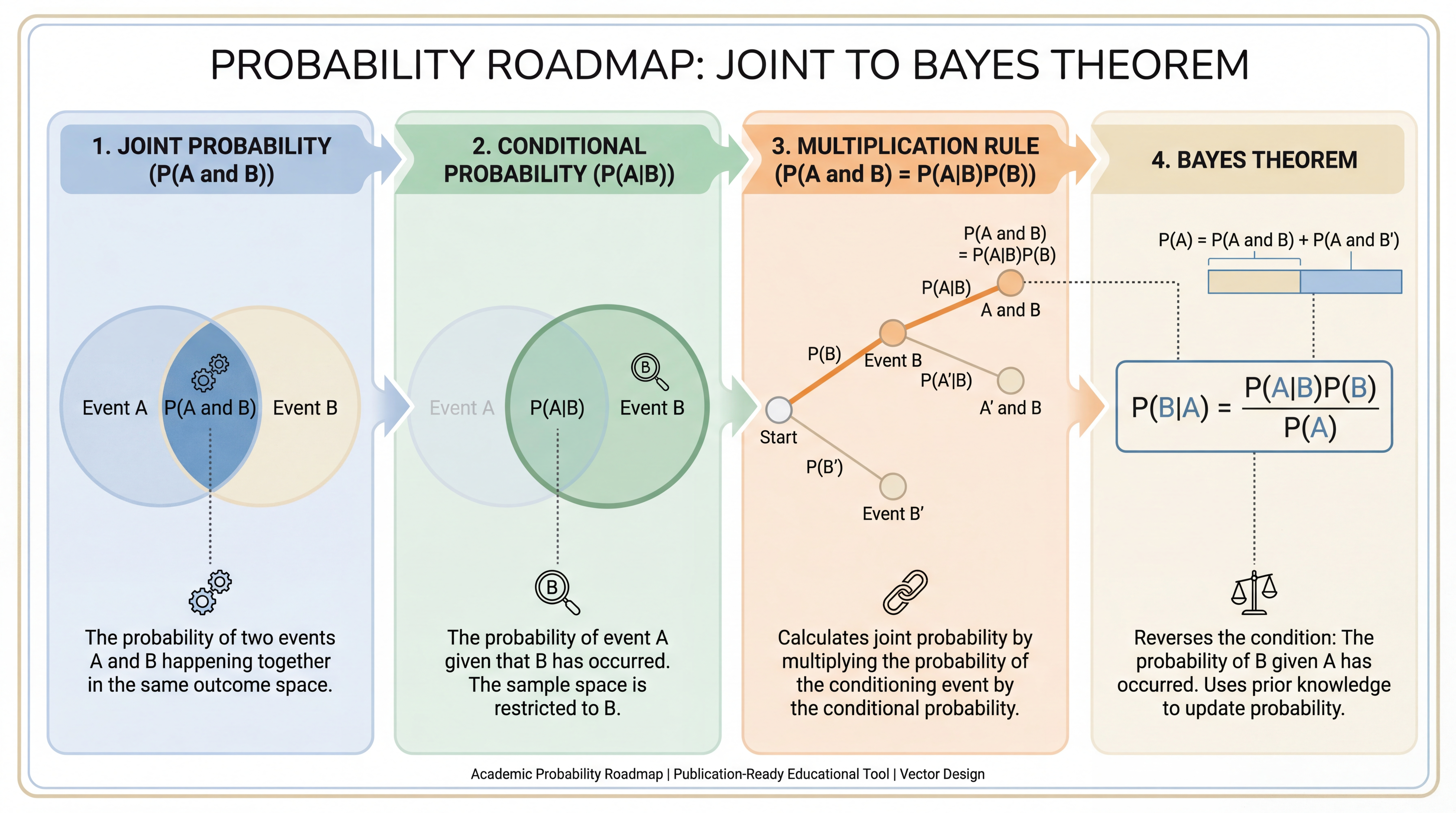
This post is a roadmap through four ideas that students often learn separately but should really understand as one connected story: joint probability, conditional probability, the multiplication rule, and finally Bayes’ theorem. The goal is to make the path feel visual, computational, and memorable.

This guide is designed to work in three ways:

• as a student-first explanation of core probability ideas
• as a NumPy-based problem-solving tutorial
• as an interview-prep guide with dropdown checks after every topic

What You Will Build Intuition For

• Why P(A and B) is the starting point for everything
• How conditional probability changes the reference group
• Why the multiplication rule is just probability bookkeeping
• How Bayes naturally falls out of the earlier ideas

One Connected Story The post does not treat joint, conditional, multiplication, and Bayes as isolated formulas.

Visible Figures The plots are shown directly, and the plotting code lives in dropdowns.

NumPy First Every major probability idea is turned into a small reproducible computation.

A light-theme infographic showing the roadmap from joint probability to conditional probability to multiplication rule to Bayes theorem with overlapping regions, a probability tree, and labeled formulas.

Learning Promise

By the end, you should be able to:

• read a joint-probability table without fear
• explain conditional probability as a change of denominator
• use the multiplication rule in both directions
• derive and apply Bayes’ theorem from earlier principles

import numpy as np
import matplotlib.pyplot as plt
from matplotlib.patches import Circle, FancyBboxPatch

plt.style.use("default")
plt.rcParams["figure.figsize"] = (8, 5)
plt.rcParams["axes.spines.top"] = False
plt.rcParams["axes.spines.right"] = False
plt.rcParams["axes.grid"] = True
plt.rcParams["grid.alpha"] = 0.18

BLUE = "#4c78a8"
ORANGE = "#f28e2b"
GREEN = "#59a14f"
RED = "#e15759"
GRAY = "#8d99ae"
LIGHT = "#eef4ff"
CREAM = "#fff6eb"
INK = "#1f2937"


def add_rounded_box(
    ax,
    x,
    y,
    width,
    height,
    text,
    facecolor,
    edgecolor="#cbd5e1",
    fontsize=11,
    text_color=INK,
    weight="bold",
):
    patch = FancyBboxPatch(
        (x, y),
        width,
        height,
        boxstyle="round,pad=0.02,rounding_size=0.04",
        linewidth=1.5,
        facecolor=facecolor,
        edgecolor=edgecolor,
    )
    ax.add_patch(patch)
    ax.text(
        x + width / 2,
        y + height / 2,
        text,
        ha="center",
        va="center",
        fontsize=fontsize,
        color=text_color,
        fontweight=weight,
        linespacing=1.25,
    )
    return patch


def setup_concept_axes(figsize):
    fig, ax = plt.subplots(figsize=figsize)
    ax.set_xlim(0, 1)
    ax.set_ylim(0, 1)
    ax.axis("off")
    return fig, ax

rng = np.random.default_rng(42)
print("NumPy version:", np.__version__)

NumPy version: 1.24.4

Part 1: Joint Probability

Q1. What is joint probability, and why does it matter so much?

Answer: Joint probability is the probability that two events happen together.

If A means “it is raining” and B means “a student carries an umbrella,” then:

\[ P(A \cap B) \]

means:

the probability that it is raining and the student carries an umbrella at the same time.

This idea matters because many later formulas are built on top of it. In fact:

• conditional probability is a joint probability divided by a reference group
• the multiplication rule rewrites a joint probability
• Bayes’ theorem comes from equating two different expressions for the same joint probability

So if you understand the overlap, you understand the foundation.

Joint probability lives in the overlap where both events are true together.

Interview Check: What is the simplest meaning of P(A ∩ B)?

It is the probability that both events happen together.

Q2. How can I see joint probability in data instead of symbols?

Answer: A two-way table is one of the best ways to build intuition.

Suppose we observe 200 days and record two binary events:

• Rain
• Umbrella

The counts are:

	Umbrella	No umbrella	Total
Rain	54	6	60
No rain	26	114	140
Total	80	120	200

From this table:

• P(Rain and Umbrella) = 54 / 200 = 0.27
• P(Rain) = 60 / 200 = 0.30
• P(Umbrella) = 80 / 200 = 0.40

counts = np.array([
    [54, 6],
    [26, 114],
])

joint = counts / counts.sum()

print("Counts table:\n", counts)
print("Joint probability table:\n", joint.round(3))
print("P(Rain and Umbrella):", round(float(joint[0, 0]), 3))
print("P(Rain):", round(float(joint[0].sum()), 3))
print("P(Umbrella):", round(float(joint[:, 0].sum()), 3))

Counts table:
 [[ 54   6]
 [ 26 114]]
Joint probability table:
 [[0.27 0.03]
 [0.13 0.57]]
P(Rain and Umbrella): 0.27
P(Rain): 0.3
P(Umbrella): 0.4

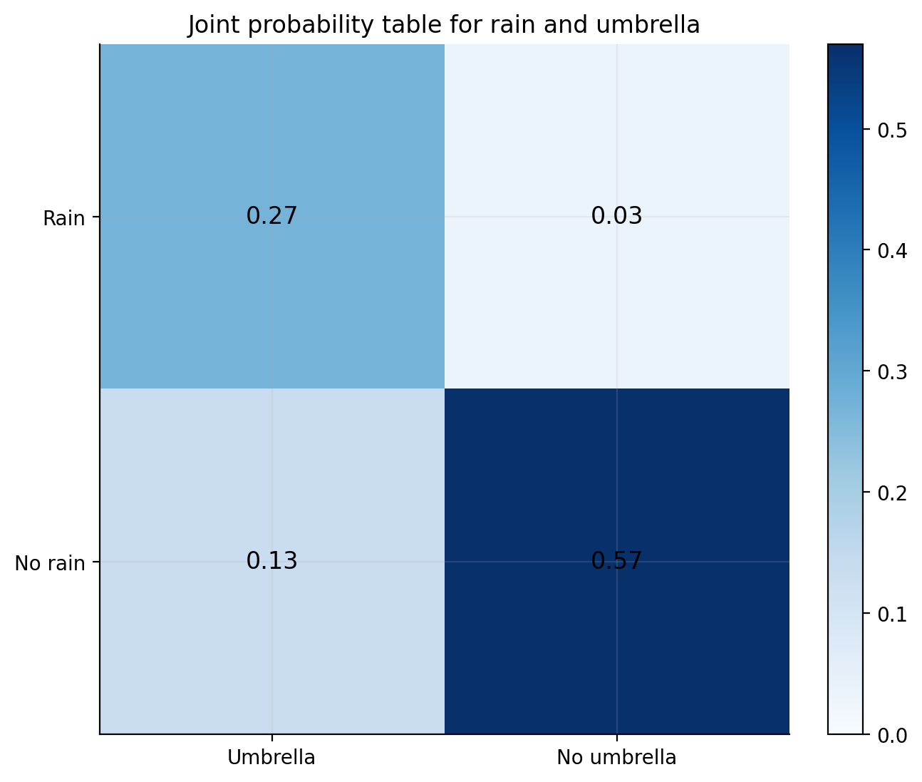
This is why tables are so useful: they let you read many probabilities from the same data.

Show Matplotlib code for this figure

fig, ax = plt.subplots(figsize=(7.4, 5.6))
im = ax.imshow(joint, cmap="Blues", vmin=0, vmax=joint.max())

for i in range(joint.shape[0]):
    for j in range(joint.shape[1]):
        ax.text(j, i, f"{joint[i, j]:.2f}", ha="center", va="center", color="black", fontsize=12)

ax.set_xticks([0, 1], labels=["Umbrella", "No umbrella"])
ax.set_yticks([0, 1], labels=["Rain", "No rain"])
ax.set_title("Joint probability table for rain and umbrella")
plt.colorbar(im, ax=ax, fraction=0.046, pad=0.04)
plt.tight_layout()
plt.show()

Interview Check: If a joint probability table sums to more than 1, what went wrong?

It is not a valid joint probability table, because all joint outcomes together must sum to 1.

Q3. How is joint probability different from independence?

Answer: Students often confuse these ideas.

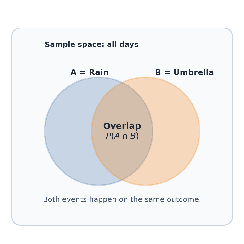
Joint probability asks:

what is the probability that both events happen together?

Independence asks:

does knowing one event change the probability of the other?

If two events are independent, then:

\[ P(A \cap B) = P(A)P(B) \]

But joint probability exists whether or not the events are independent.

For the rain and umbrella table:

• P(Rain) = 0.30
• P(Umbrella) = 0.40
• if they were independent, P(Rain and Umbrella) would be 0.30 x 0.40 = 0.12
• the actual joint probability is 0.27

That is much larger, so umbrella carrying is clearly not independent of rain.

p_rain = joint[0].sum()
p_umbrella = joint[:, 0].sum()
p_joint_actual = joint[0, 0]
p_joint_if_independent = p_rain * p_umbrella

print("Actual joint probability:", round(float(p_joint_actual), 3))
print("Joint probability if independent:", round(float(p_joint_if_independent), 3))

Actual joint probability: 0.27
Joint probability if independent: 0.12

Interview Check: Does a joint probability automatically imply independence?

No. Joint probability only describes the overlap; independence is a separate relationship about whether one event changes the probability of the other.

Part 2: Conditional Probability

Q4. What does conditional probability actually mean?

Answer: Conditional probability means we restrict attention to a smaller world where one event is already known to be true.

For example:

\[ P(Rain \mid Umbrella) \]

means:

if I only look at days when an umbrella was carried, what fraction of those days were rainy?

That is the key mental move:

• ordinary probability divides by all cases
• conditional probability divides by a restricted set of cases

From the table above:

• total umbrella days = 80
• rainy umbrella days = 54

So:

\[ P(Rain \mid Umbrella) = \frac{54}{80} = 0.675 \]

p_rain_given_umbrella = joint[0, 0] / joint[:, 0].sum()
p_umbrella_given_rain = joint[0, 0] / joint[0].sum()

print("P(Rain | Umbrella):", round(float(p_rain_given_umbrella), 3))
print("P(Umbrella | Rain):", round(float(p_umbrella_given_rain), 3))

P(Rain | Umbrella): 0.675
P(Umbrella | Rain): 0.9

These two are not the same. One conditions on umbrella days; the other conditions on rainy days.

Conditional probability restricts attention to the conditioned world first, then measures the overlap inside it.

Interview Check: What changes when we move from P(A) to P(A|B)?

The denominator changes from all cases to only the cases where B is true.

Q5. Why is conditional probability often called a change of denominator?

Answer: Because that is exactly what happens mathematically.

For any two events A and B:

\[ P(A \mid B) = \frac{P(A \cap B)}{P(B)} \]

The numerator is the overlap. The denominator is the new reference group.

This is one of the most important formulas in probability because it explains the meaning of the vertical bar |.

If B becomes your world, then only outcomes inside B count.

In the umbrella example:

• P(Rain and Umbrella) = 54 / 200
• P(Umbrella) = 80 / 200

So:

\[ P(Rain \mid Umbrella) = \frac{54/200}{80/200} = \frac{54}{80} \]

The total number of all days disappears because the condition changes the reference group.

Interview Check: Why does P(A|B) divide by P(B) instead of P(A)?

Because once B is known to be true, the probability is measured only within the B cases.

Q6. Can I make conditional probability visual?

Answer: Yes. A simple bar-style restriction view helps a lot.

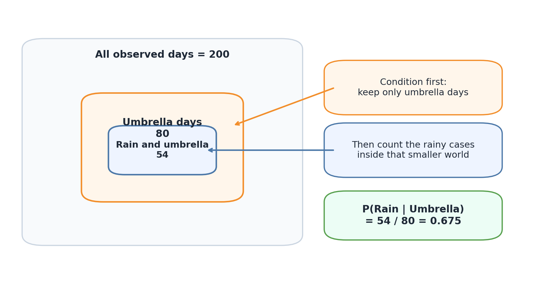
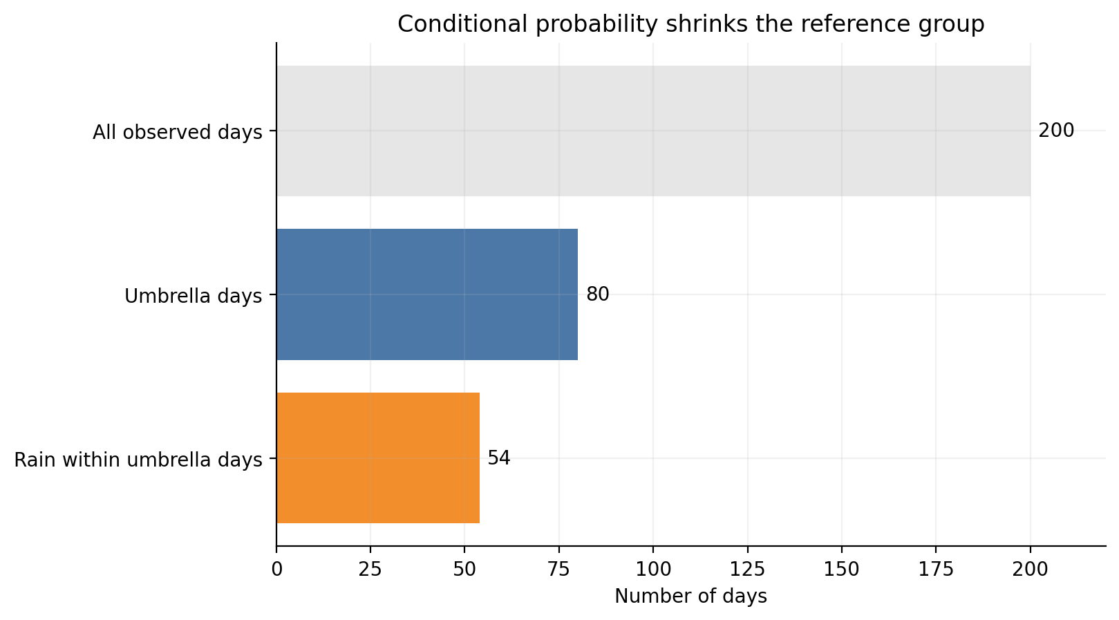
Think of all 200 days as one big bar. The umbrella days are a smaller highlighted section of that bar. Inside that highlighted section, the rainy umbrella days form the part that counts toward P(Rain | Umbrella).

Show Matplotlib code for this figure

all_days = counts.sum()
umbrella_days = counts[:, 0].sum()
rain_and_umbrella = counts[0, 0]
y_positions = np.array([2, 1, 0])
labels = ["All observed days", "Umbrella days", "Rain within umbrella days"]
values = np.array([all_days, umbrella_days, rain_and_umbrella])

fig, ax = plt.subplots(figsize=(8.2, 4.6))
ax.barh(y_positions, values, color=["#e6e6e6", BLUE, ORANGE], edgecolor="none")

for y, value in zip(y_positions, values):
    ax.text(value + 2, y, str(int(value)), va="center", fontsize=10)

ax.set_xlim(0, 220)
ax.set_yticks(y_positions, labels=labels)
ax.set_xlabel("Number of days")
ax.set_title("Conditional probability shrinks the reference group")
plt.tight_layout()
plt.show()

Interview Check: In P(Rain|Umbrella), what is the new reference group?

The reference group is all umbrella days.

Q7. Why are P(A|B) and P(B|A) usually different?

Answer: Because they condition on different worlds.

Using the same table:

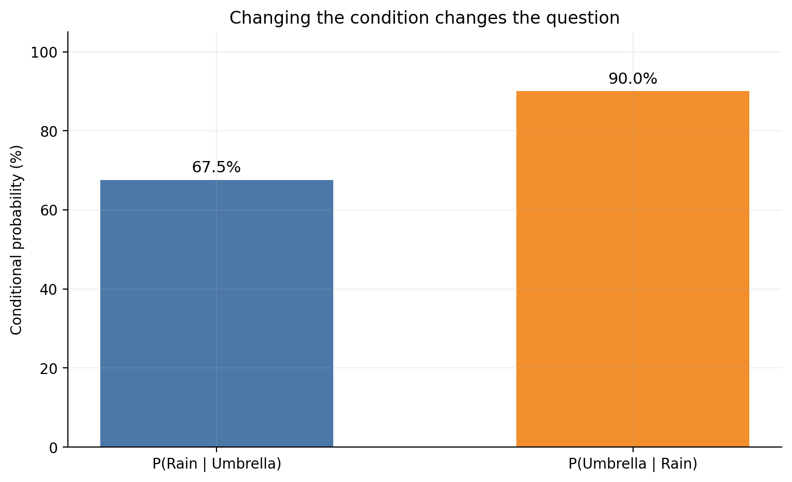
• P(Rain | Umbrella) = 54 / 80 = 0.675
• P(Umbrella | Rain) = 54 / 60 = 0.900

Those are both correct, but they answer different questions:

• among umbrella days, how many were rainy?
• among rainy days, how many had umbrellas?

This is one of the most common sources of confusion in interview questions. The symbol order is not cosmetic. It changes the denominator and therefore changes the meaning.

comparison = np.array([p_rain_given_umbrella, p_umbrella_given_rain])
print("Comparison:", comparison.round(3))

Comparison: [0.675 0.9  ]

Show Matplotlib code for this figure

fig, ax = plt.subplots(figsize=(7.8, 4.8))
bars = ax.bar(
    ["P(Rain | Umbrella)", "P(Umbrella | Rain)"],
    comparison * 100,
    color=[BLUE, ORANGE],
    width=0.56
)

for bar, value in zip(bars, comparison * 100):
    ax.text(bar.get_x() + bar.get_width() / 2, value + 2, f"{value:.1f}%", ha="center", fontsize=11)

ax.set_ylabel("Conditional probability (%)")
ax.set_ylim(0, 105)
ax.set_title("Changing the condition changes the question")
plt.tight_layout()
plt.show()

Interview Check: Why is P(A|B) usually not equal to P(B|A)?

Because the conditioning event changes the denominator, so the two expressions are measured on different reference groups.

Part 3: The Multiplication Rule

Q8. What is the multiplication rule, and where does it come from?

Answer: The multiplication rule is just a rearrangement of conditional probability.

Starting from:

\[ P(A \mid B) = \frac{P(A \cap B)}{P(B)} \]

Multiply both sides by P(B):

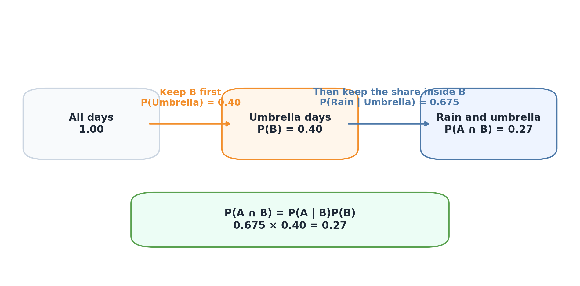
\[ P(A \cap B) = P(A \mid B)P(B) \]

You can also write:

\[ P(A \cap B) = P(B \mid A)P(A) \]

This rule is not a new idea. It is the same overlap described in a different way.

In the umbrella example:

\[ P(Rain \cap Umbrella) = P(Rain \mid Umbrella)P(Umbrella) \]

and also:

\[ P(Rain \cap Umbrella) = P(Umbrella \mid Rain)P(Rain) \]

Both equal the same joint probability.

left = joint[0, 0]
right_1 = p_rain_given_umbrella * p_umbrella
right_2 = p_umbrella_given_rain * p_rain

print("Joint probability:", round(float(left), 3))
print("P(Rain | Umbrella) * P(Umbrella):", round(float(right_1), 3))
print("P(Umbrella | Rain) * P(Rain):", round(float(right_2), 3))

Joint probability: 0.27
P(Rain | Umbrella) * P(Umbrella): 0.27
P(Umbrella | Rain) * P(Rain): 0.27

The multiplication rule keeps one event first, then keeps the share of that event where the second event is true.

Interview Check: Is the multiplication rule a completely new formula, or a rearrangement of conditional probability?

It is a rearrangement of the conditional probability formula.

Q9. How does the multiplication rule help with sequential events?

Answer: It becomes especially useful when events happen in sequence.

Imagine drawing cards from a deck without replacement:

• Event A: first card is an ace
• Event B: second card is a king given the first card was an ace

Then:

\[ P(A \cap B) = P(A)P(B \mid A) \]

Because the second probability depends on what happened first.

p_first_ace = 4 / 52
p_second_king_given_first_ace = 4 / 51
p_ace_then_king = p_first_ace * p_second_king_given_first_ace

print("P(first ace):", round(p_first_ace, 5))
print("P(second king | first ace):", round(p_second_king_given_first_ace, 5))
print("P(first ace and second king):", round(p_ace_then_king, 5))

P(first ace): 0.07692
P(second king | first ace): 0.07843
P(first ace and second king): 0.00603

This is why the multiplication rule is so useful: it turns a complex sequence into a product of manageable steps.

Interview Check: Why is P(B|A) necessary in sequential problems?

Because the probability of the later event may depend on what happened earlier.

Q10. Can I visualize the multiplication rule with a probability tree?

Answer: Yes. A probability tree makes path probabilities feel natural.

Each branch stores a conditional probability, and the probability of a full path is the product of the branch probabilities along that path.

Here is a tree for the rain-and-umbrella example:

• first split by Rain vs No rain
• then split each branch by Umbrella vs No umbrella

Show Matplotlib code for this figure

fig, ax = plt.subplots(figsize=(9.2, 5.6))
ax.axis("off")

nodes = {
    "start": (0.06, 0.5),
    "rain": (0.36, 0.76),
    "no_rain": (0.36, 0.24),
    "rain_umb": (0.74, 0.88),
    "rain_no": (0.74, 0.64),
    "no_rain_umb": (0.74, 0.36),
    "no_rain_no": (0.74, 0.12),
}

edges = [
    ("start", "rain", f"P(Rain) = {p_rain:.2f}", BLUE),
    ("start", "no_rain", f"P(No rain) = {1 - p_rain:.2f}", GRAY),
    ("rain", "rain_umb", f"P(Umbrella | Rain) = {p_umbrella_given_rain:.2f}", ORANGE),
    ("rain", "rain_no", f"P(No umbrella | Rain) = {1 - p_umbrella_given_rain:.2f}", GRAY),
    ("no_rain", "no_rain_umb", f"P(Umbrella | No rain) = {joint[1,0] / (1-p_rain):.2f}", BLUE),
    ("no_rain", "no_rain_no", f"P(No umbrella | No rain) = {joint[1,1] / (1-p_rain):.2f}", GREEN),
]

for src, dst, label, color in edges:
    x1, y1 = nodes[src]
    x2, y2 = nodes[dst]
    ax.plot([x1, x2], [y1, y2], color=color, linewidth=2.5)
    ax.text((x1 + x2) / 2, (y1 + y2) / 2 + 0.03, label, fontsize=9, ha="center")

for name, (x, y) in nodes.items():
    ax.scatter([x], [y], s=170, color="white", edgecolor="#334155", linewidth=1.2, zorder=3)

ax.text(*nodes["start"], "Start", ha="center", va="center")
ax.text(*nodes["rain"], "Rain", ha="center", va="center")
ax.text(*nodes["no_rain"], "No rain", ha="center", va="center")
ax.text(*nodes["rain_umb"], "Rain & Umbrella\n0.27", ha="center", va="center")
ax.text(*nodes["rain_no"], "Rain & No umbrella\n0.03", ha="center", va="center")
ax.text(*nodes["no_rain_umb"], "No rain & Umbrella\n0.13", ha="center", va="center")
ax.text(*nodes["no_rain_no"], "No rain & No umbrella\n0.57", ha="center", va="center")

ax.set_title("Probability trees turn joint probability into a path product", pad=14)
plt.tight_layout()
plt.show()

Interview Check: What do you multiply along a probability tree path?

You multiply the conditional branch probabilities along that path.

Q11. What happens when there are three events instead of two?

Answer: The same logic keeps extending.

For three events:

\[ P(A \cap B \cap C) = P(A)\,P(B \mid A)\,P(C \mid A \cap B) \]

This is sometimes called a simple case of the chain rule of probability.

The idea is straightforward:

• first event probability
• second event conditional on the first
• third event conditional on the first two

That keeps going for longer sequences.

p_a = 0.6
p_b_given_a = 0.5
p_c_given_ab = 0.2
p_abc = p_a * p_b_given_a * p_c_given_ab

print("P(A and B and C):", round(p_abc, 4))

P(A and B and C): 0.06

This matters because many real problems are built from staged dependencies rather than one-shot events.

Interview Check: In the three-event chain rule, what does the last factor represent?

It represents the probability of the third event given that the earlier events have already happened.

Part 4: From Multiplication to Bayes

Q12. How do we derive Bayes’ theorem from the multiplication rule?

Answer: Bayes’ theorem appears when you write the same joint probability in two ways.

For events A and B:

\[ P(A \cap B) = P(A \mid B)P(B) \]

and also:

\[ P(A \cap B) = P(B \mid A)P(A) \]

Since both equal the same joint probability, set them equal:

\[ P(A \mid B)P(B) = P(B \mid A)P(A) \]

Now divide by P(B):

\[ P(A \mid B) = \frac{P(B \mid A)P(A)}{P(B)} \]

That is Bayes’ theorem.

This is why Bayes should not feel like a disconnected formula. It is a direct consequence of earlier probability ideas.

Interview Check: What single idea is Bayes’ theorem built from most directly?

It comes from equating two multiplication-rule expressions for the same joint probability.

Q13. What do prior, likelihood, evidence, and posterior mean in Bayes’ theorem?

Answer: These words turn the formula into a story.

\[ P(A \mid B) = \frac{P(B \mid A)P(A)}{P(B)} \]

If we rename the terms:

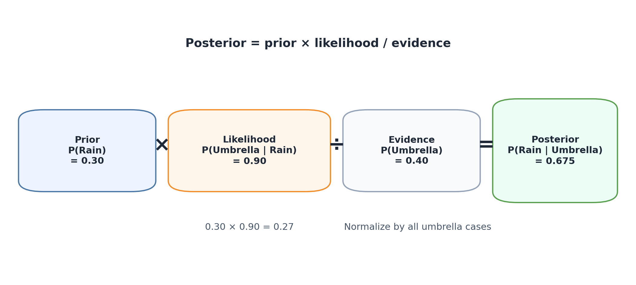
• P(A) = prior
• P(B|A) = likelihood
• P(B) = evidence
• P(A|B) = posterior

then Bayes becomes:

posterior = likelihood x prior / evidence

This language matters because it helps you map real problems onto the formula.

For example:

• hypothesis = “it is raining”
• evidence = “an umbrella is observed”
• prior = how common rain is overall
• likelihood = how likely umbrellas are when it rains
• posterior = how likely rain is after seeing an umbrella

From our table:

posterior_rain_given_umbrella = p_umbrella_given_rain * p_rain / p_umbrella
print("Posterior P(Rain | Umbrella):", round(float(posterior_rain_given_umbrella), 3))

Posterior P(Rain | Umbrella): 0.675

Bayes’ theorem reweights the prior by the likelihood and then normalizes by the total evidence.

Interview Check: In Bayes’ theorem, what role does the evidence term play?

It normalizes the numerator by the total probability of the observed evidence.

Q14. Why is Bayes’ theorem so useful in real reasoning?

Answer: Because in real life we often observe the evidence first and want to reason backward to the hidden cause.

We rarely care only about:

• P(Umbrella | Rain)

We usually care more about:

• P(Rain | Umbrella)

That reversal is exactly what Bayes gives us.

This is why Bayes appears in:

• diagnosis
• spam filtering
• fault detection
• search ranking
• machine learning classification

The broad pattern is always the same:

1. there is a hidden state
2. there is an observable clue
3. we want to infer the hidden state from the clue

That is Bayesian reasoning in one sentence.

Interview Check: Why is Bayes often described as reasoning backward from evidence to cause?

Because it helps us start from an observed clue and infer how likely a hidden explanation is.

Part 5: Bayes in Practice

Q15. How does this look in a medical-testing example?

Answer: Medical testing is the classic Bayes example because it separates:

• the test behavior
• the disease prevalence
• the final posterior after seeing a result

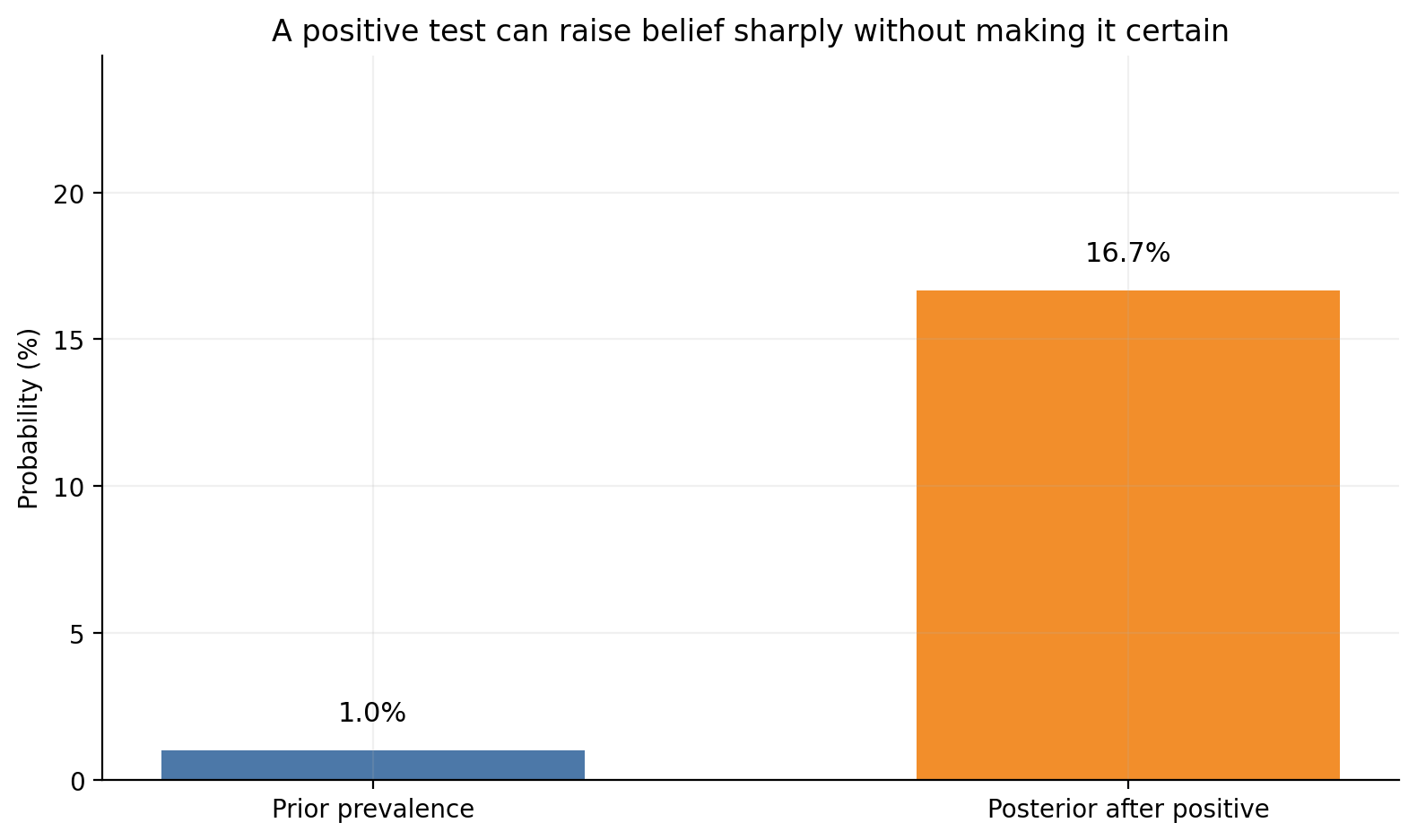
Suppose:

• disease prevalence = 1%
• sensitivity = 99%
• specificity = 95%

Then:

prior = 0.01
sensitivity = 0.99
specificity = 0.95

posterior_positive = sensitivity * prior / (
    sensitivity * prior + (1 - specificity) * (1 - prior)
)

print(f"Prior probability of disease: {prior:.2%}")
print(f"Posterior after a positive test: {posterior_positive:.2%}")

Prior probability of disease: 1.00%
Posterior after a positive test: 16.67%

This usually surprises students. A very accurate test does not automatically mean a positive result implies near-certain disease. The base rate still matters.

Show Matplotlib code for this figure

fig, ax = plt.subplots(figsize=(8, 4.8))
values = np.array([prior * 100, posterior_positive * 100])
bars = ax.bar(["Prior prevalence", "Posterior after positive"], values, color=[BLUE, ORANGE], width=0.56)

for bar, value in zip(bars, values):
    ax.text(bar.get_x() + bar.get_width() / 2, value + 1, f"{value:.1f}%", ha="center", fontsize=11)

ax.set_ylabel("Probability (%)")
ax.set_ylim(0, max(values) + 8)
ax.set_title("A positive test can raise belief sharply without making it certain")
plt.tight_layout()
plt.show()

Interview Check: Why does a positive test result not automatically imply a very high posterior?

Because the posterior also depends on the base rate and the false-positive behavior of the test.

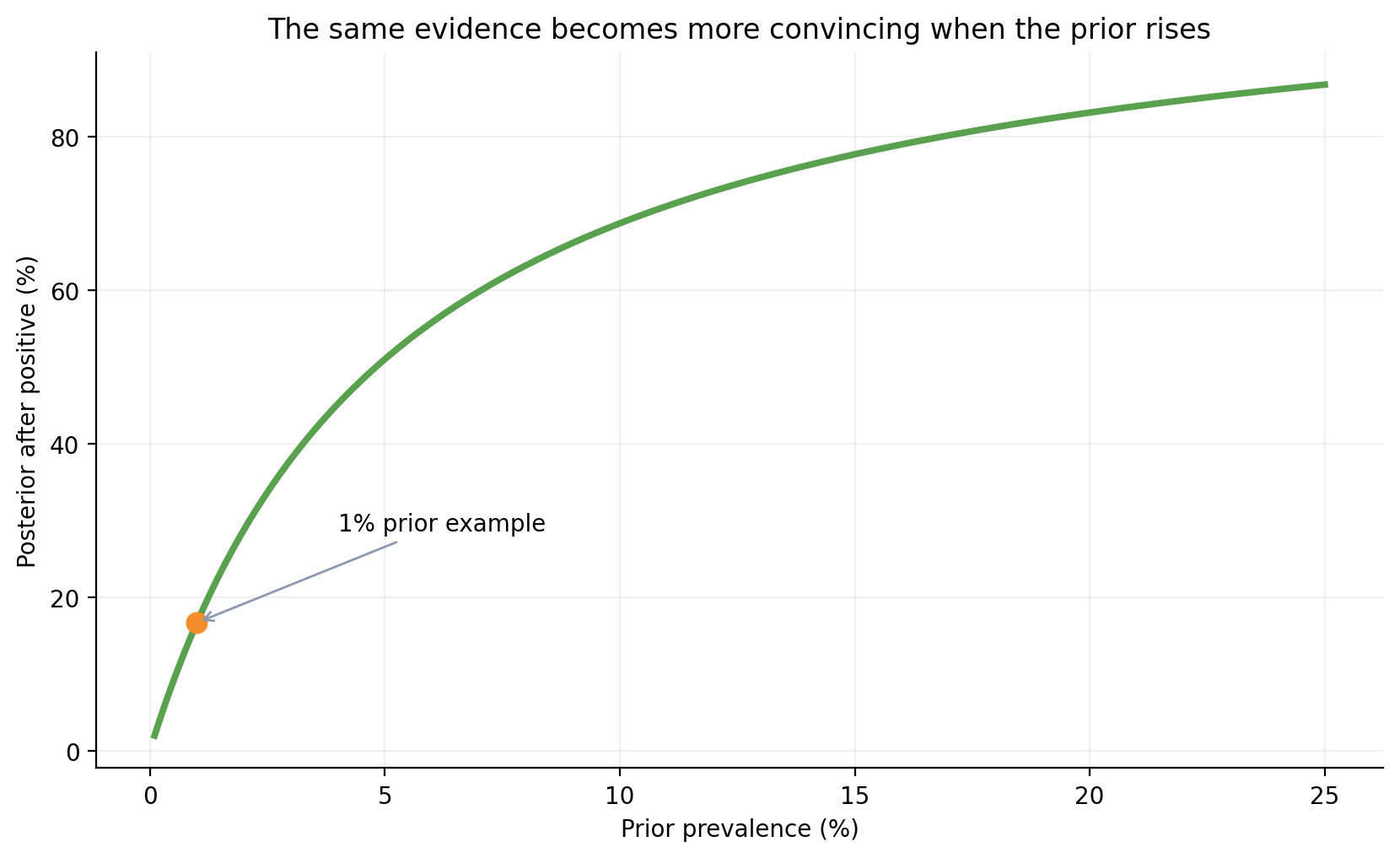
Q16. How does the prior change what the same evidence means?

Answer: The same test result can mean very different things under different priors.

That is one of the deepest Bayes ideas:

evidence never acts alone; it updates whatever belief you started with.

priors = np.linspace(0.001, 0.25, 300)
posterior_curve = sensitivity * priors / (
    sensitivity * priors + (1 - specificity) * (1 - priors)
)

print("Posterior at 1% prior:", round(float(posterior_curve[np.argmin(np.abs(priors - 0.01))]), 4))
print("Posterior at 10% prior:", round(float(posterior_curve[np.argmin(np.abs(priors - 0.10))]), 4))

Posterior at 1% prior: 0.1689
Posterior at 10% prior: 0.6877

Show Matplotlib code for this figure

fig, ax = plt.subplots(figsize=(8.4, 5.2))
ax.plot(priors * 100, posterior_curve * 100, color=GREEN, linewidth=2.8)
ax.scatter([1], [posterior_positive * 100], color=ORANGE, s=70, zorder=3)
ax.annotate("1% prior example", (1, posterior_positive * 100), xytext=(4, posterior_positive * 100 + 12),
            arrowprops=dict(arrowstyle="->", color=GRAY), fontsize=10)
ax.set_xlabel("Prior prevalence (%)")
ax.set_ylabel("Posterior after positive (%)")
ax.set_title("The same evidence becomes more convincing when the prior rises")
plt.tight_layout()
plt.show()

Interview Check: Why can the same evidence lead to different posteriors in different settings?

Because Bayes combines the evidence with the starting prior, so different starting beliefs update to different final beliefs.

Q17. How can I implement Bayes for multiple hypotheses with NumPy?

Answer: Bayes is not limited to one hypothesis versus its complement. NumPy makes it easy to compare many hypotheses at once.

Suppose you have three possible causes and one observed clue:

hypotheses = np.array(["Cause A", "Cause B", "Cause C"])
priors_multi = np.array([0.5, 0.3, 0.2])
likelihoods_multi = np.array([0.1, 0.7, 0.4])

unnormalized = priors_multi * likelihoods_multi
posterior_multi = unnormalized / unnormalized.sum()

print("Posterior:", posterior_multi.round(4))
print("Most likely hypothesis:", hypotheses[np.argmax(posterior_multi)])

Posterior: [0.1471 0.6176 0.2353]
Most likely hypothesis: Cause B

This is the same pattern as before:

1. multiply prior by likelihood
2. add the raw scores to get the evidence
3. divide through to normalize

That simple three-line pattern is the computational heart of many Bayesian updates.

Interview Check: Why do we divide by unnormalized.sum() in the multi-hypothesis case?

Because the raw prior-times-likelihood scores must be normalized so the posterior probabilities sum to 1.

Q18. What practical workflow should I use in exams or interviews?

Answer: A clean workflow reduces mistakes.

Use this sequence:

1. Define the events or the hypothesis and evidence clearly.
2. Decide whether the problem is asking for a joint probability, a conditional probability, a multiplication-rule expression, or a Bayes update.
3. Write the correct denominator before plugging numbers in.
4. Check whether the result is supposed to be a probability of an overlap, a restricted group, or an updated belief.
5. Do a sanity check.

Useful sanity checks:

• probabilities must stay between 0 and 1
• a full joint table must sum to 1
• conditioning should usually change the denominator
• if evidence strongly favors a hypothesis, the posterior should rise

This habit is often the difference between understanding and memorizing.

Interview Check: What is the best first move in a probability word problem?

Clearly define the events and identify what type of probability the question is asking for.

Part 6: Deeper Foundations and Common Mistakes

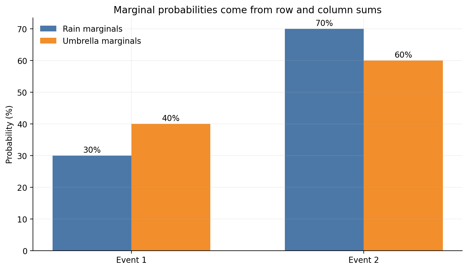
Q19. What are marginal probabilities, and why do row and column sums matter?

Answer: Marginal probabilities are the probabilities of one event alone, obtained by summing across the other event’s possibilities in a joint table.

From the rain-and-umbrella table:

• row sums give P(Rain) and P(No rain)
• column sums give P(Umbrella) and P(No umbrella)

That is why the word marginal is used. In textbook tables, these totals are often written in the margins.

Marginals matter because:

• conditional probability divides by them
• independence compares the joint probability against their product
• Bayes uses them through the evidence term

row_marginals = joint.sum(axis=1)
col_marginals = joint.sum(axis=0)

print("Row marginals [Rain, No rain]:", row_marginals.round(3))
print("Column marginals [Umbrella, No umbrella]:", col_marginals.round(3))

Row marginals [Rain, No rain]: [0.3 0.7]
Column marginals [Umbrella, No umbrella]: [0.4 0.6]

Show Matplotlib code for this figure

fig, ax = plt.subplots(figsize=(8.2, 4.8))
x = np.arange(2)
width = 0.34

bars1 = ax.bar(x - width / 2, row_marginals * 100, width, label="Rain marginals", color=BLUE)
bars2 = ax.bar(x + width / 2, col_marginals * 100, width, label="Umbrella marginals", color=ORANGE)

ax.set_xticks(x, labels=["Event 1", "Event 2"])
ax.set_ylabel("Probability (%)")
ax.set_title("Marginal probabilities come from row and column sums")
ax.legend(frameon=False)

for bars in (bars1, bars2):
    for bar in bars:
        ax.text(bar.get_x() + bar.get_width() / 2, bar.get_height() + 1, f"{bar.get_height():.0f}%", ha="center", fontsize=10)

plt.tight_layout()
plt.show()

Interview Check: What is a marginal probability in a joint table?

It is the probability of one event alone, obtained by summing over the other variable’s possibilities.

Q20. What is the law of total probability, and why does it matter for Bayes?

Answer: The law of total probability says that if an event can happen through several mutually exclusive routes, then the total probability is the sum of those route probabilities.

For two routes, A and not A:

\[ P(B) = P(B \mid A)P(A) + P(B \mid \neg A)P(\neg A) \]

In the umbrella example:

\[ P(Umbrella) = P(Umbrella \mid Rain)P(Rain) + P(Umbrella \mid No\ rain)P(No\ rain) \]

This is important because the Bayes denominator is often computed exactly this way.

p_umbrella_given_no_rain = joint[1, 0] / joint[1].sum()
umbrella_via_total_probability = p_umbrella_given_rain * p_rain + p_umbrella_given_no_rain * (1 - p_rain)

print("P(Umbrella) directly:", round(float(p_umbrella), 3))
print("P(Umbrella) via total probability:", round(float(umbrella_via_total_probability), 3))

P(Umbrella) directly: 0.4
P(Umbrella) via total probability: 0.4

The conceptual lesson is simple:

• list all mutually exclusive routes
• compute the probability of each route
• add them to get the total

That habit is one of the best ways to avoid Bayes denominator mistakes.

Interview Check: Why is the law of total probability closely tied to Bayes’ theorem?

Because it is often the method used to compute the evidence term in the Bayes denominator.

Q21. What is the difference between independence and conditional independence?

Answer: Independence means:

\[ P(A \cap B) = P(A)P(B) \]

Conditional independence means:

\[ P(A \cap B \mid C) = P(A \mid C)P(B \mid C) \]

So the difference is:

• independence is a claim in the full probability space
• conditional independence is a claim only after some condition C is known

This is a very important distinction in probabilistic modeling. Naive Bayes, for example, does not assume features are fully independent in all situations. It assumes they are approximately independent given the class.

That is a weaker and more structured claim than ordinary independence.

Interview Check: What extra ingredient appears in conditional independence but not ordinary independence?

A conditioning event or variable, meaning the independence claim is made only after that condition is fixed.

Q22. What mistakes do students make most often across these topics?

Answer: Most mistakes come from mixing up the meaning of the denominator.

The most common ones are:

1. confusing a joint probability with a conditional probability
2. mixing up P(A|B) and P(B|A)
3. reading a single cell when the problem actually needs a row sum or column sum
4. assuming independence without justification
5. forgetting to compute the evidence term in Bayes problems
6. dividing by all cases when the condition should restrict the denominator

One good rule of thumb is:

before computing anything, say out loud what your denominator represents.

That simple habit dramatically improves accuracy.

Interview Check: What is the most common denominator mistake in conditional-probability problems?

Students often divide by all cases instead of dividing by only the cases that satisfy the condition.

---

Quick Interview Round

1. What does P(A ∩ B) represent?

It represents the probability that both events happen together.

2. Why is a two-way table useful in probability?

Because it lets you read joint, marginal, and conditional probabilities from the same data.

3. What is a marginal probability?

It is the probability of one event alone, obtained by summing over the other event’s possibilities.

4. How can you tell from numbers that two events are not independent?

If the actual joint probability is different from the product of the marginals, the events are not independent.

5. What is the intuitive meaning of the vertical bar in P(A|B)?

It means “given that,” so the probability is measured in the restricted world where B is true.

6. Why does conditional probability change the denominator?

Because once the condition is known, only the cases satisfying that condition remain in the reference group.

7. Why are P(A|B) and P(B|A) usually different?

Because they condition on different events and therefore use different denominators.

8. What does the multiplication rule compute?

It computes a joint probability using a marginal probability and a conditional probability.

9. When is the multiplication rule especially useful?

It is especially useful in sequential problems where later events depend on earlier ones.

10. What do you multiply on a probability tree?

You multiply the branch probabilities along the path of interest.

11. How does the chain rule extend the multiplication rule?

It applies the same logic repeatedly for three or more dependent events.

12. What is the quickest derivation of Bayes’ theorem?

Write the same joint probability in two multiplication-rule forms and solve for the desired conditional probability.

13. What is the prior in Bayes’ theorem?

It is the belief about the hypothesis before the new evidence is observed.

14. What is the likelihood in Bayes’ theorem?

It is the probability of the evidence assuming the hypothesis is true.

15. What is the evidence term in Bayes’ theorem?

It is the total probability of the observed evidence across all relevant ways the evidence can occur.

16. What is the posterior?

It is the updated belief about the hypothesis after incorporating the evidence.

17. Why does a rare disease create counterintuitive Bayes results?

Because even accurate tests can produce many false positives when the healthy population is much larger than the sick population.

18. Why is NumPy useful for Bayesian calculations?

Because it makes it easy to represent priors, likelihoods, and normalized posteriors as arrays.

19. What is a strong sanity check after computing a posterior over several hypotheses?

Check that the posterior entries are non-negative and sum to 1.

20. What connects joint probability, conditional probability, the multiplication rule, and Bayes into one story?

They are all different ways of describing how events overlap and how evidence changes what part of the probability space we focus on.

21. Why are marginal probabilities called marginals?

Because they are obtained by summing rows or columns and are often written in the margins of a table.

22. What does the law of total probability usually help compute in Bayes problems?

It usually helps compute the total probability of the evidence, which becomes the Bayes denominator.

23. What is the main difference between independence and conditional independence?

Conditional independence only claims independence after some third condition is known.

24. Why is identifying the denominator often the key step in probability problems?

Because the denominator tells you what reference group the probability is being measured over.

25. In a joint table, when should you sum instead of reading a single cell?

You should sum when the question asks for a marginal or total probability across several outcomes rather than one exact overlap.

---

Summary

The cleanest way to understand this topic is to see it as a progression:

• joint probability describes overlap
• conditional probability changes the reference group
• the multiplication rule rewrites the overlap in a useful way
• Bayes’ theorem turns observed evidence into updated belief
• marginals and total probability organize the bookkeeping behind the formulas
• conditional independence explains why some probabilistic models stay useful

If that ladder feels natural, then the formulas stop looking disconnected. They become different views of the same underlying structure.

---

References

1. 3Blue1Brown: Bayes’ Theorem
2. Machine Learning Mastery: A Gentle Introduction to Bayes Theorem for Machine Learning