Multi-Layer Perceptrons: From Mathematics to Implementation
A complete guide to understanding neural networks from first principles
Deep Learning
Neural Networks
Machine Learning
Tutorial
Author
Rishabh Mondal
Published
February 18, 2025
Welcome to the World of Neural Networks!
This tutorial will take you on a journey from understanding the basic concepts of neural networks to implementing a fully functional Multi-Layer Perceptron (MLP) from scratch. We’ll use pure mathematics first, then build intuition with hand calculations, and finally implement everything in Python with NumPy.
Matrix-first approach: Understand the mathematics before writing code
Hand calculations: Work through examples step-by-step
From scratch implementation: No ML libraries, just NumPy
Real dataset training: See your network learn!
Prerequisites: Basic Python, linear algebra (matrices), and calculus (derivatives)
Part 1: The Big Picture (Easy)
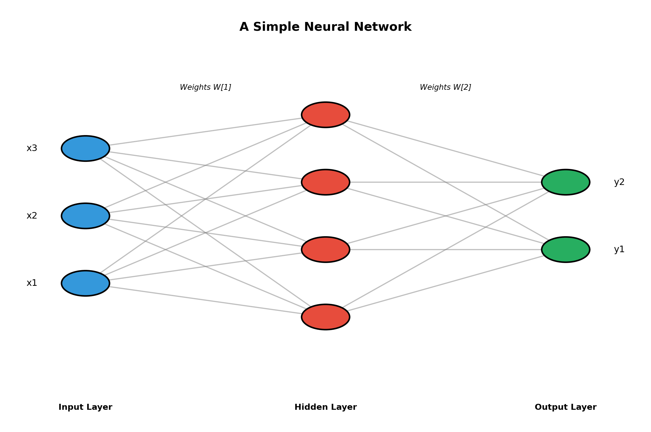
1.1 What is a Neural Network?
A neural network is a computational model inspired by the human brain. Just as our brains have billions of neurons connected together, artificial neural networks have computational units (nodes) connected in layers.
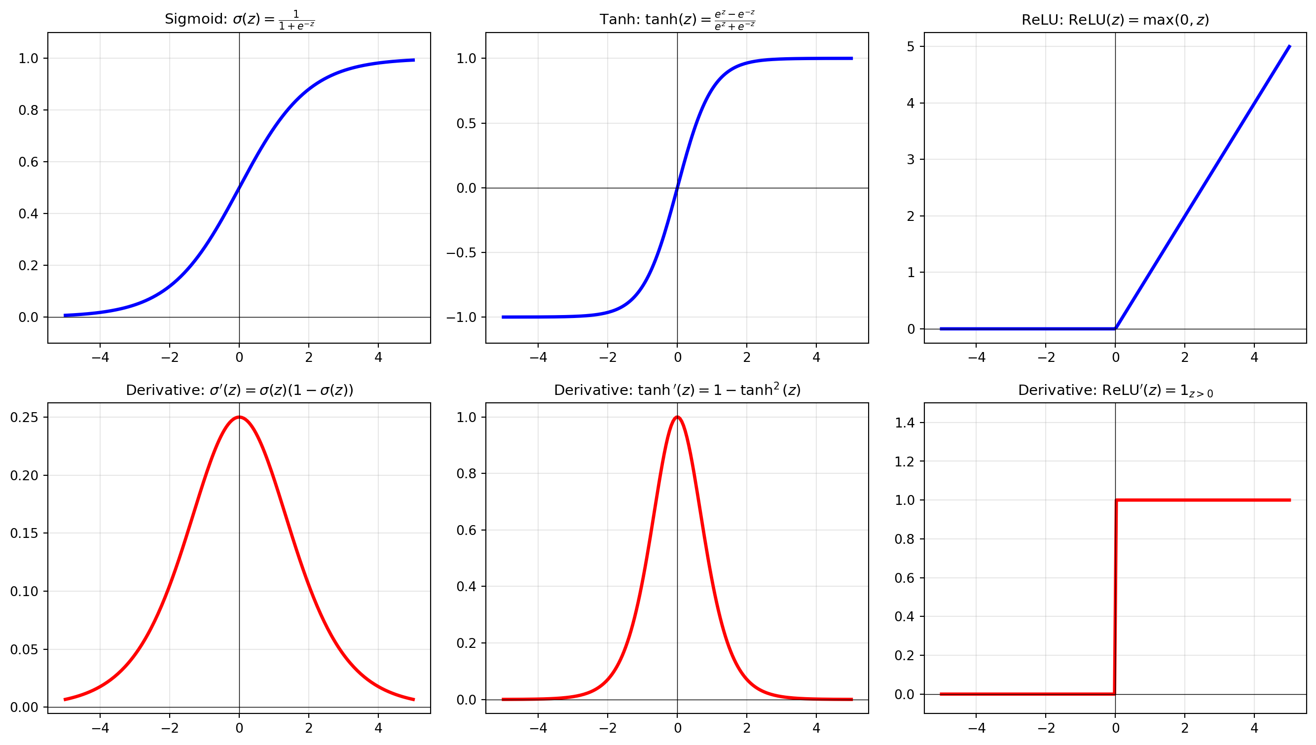
Without activation functions, a neural network is just a series of linear transformations: \[y = W_2(W_1 x + b_1) + b_2 = W_2 W_1 x + W_2 b_1 + b_2 = W' x + b'\]
This collapses to a single linear transformation! Activation functions introduce non-linearity, allowing the network to learn complex patterns.
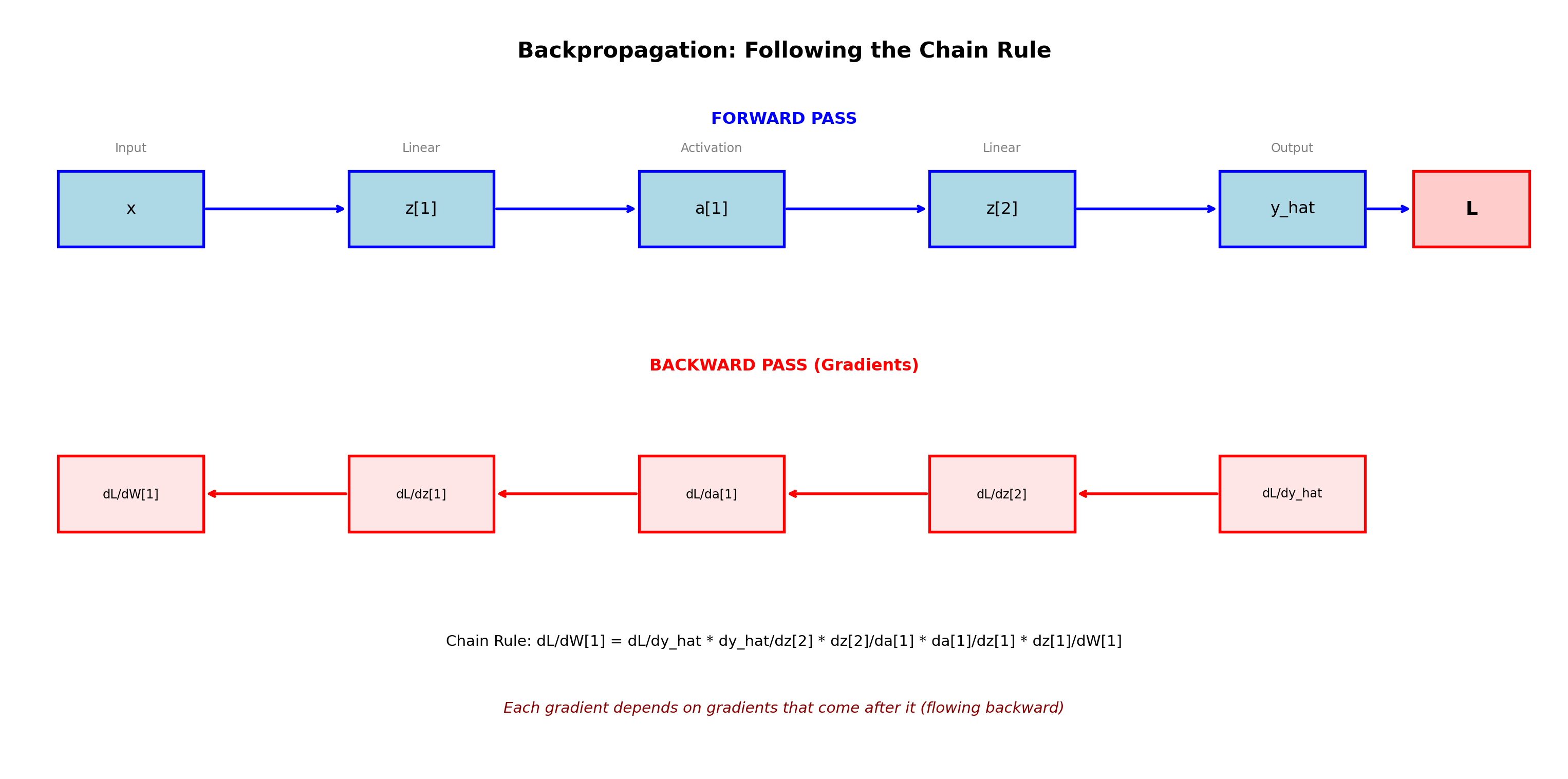
Part 3: Backpropagation - Learning from Mistakes (Moderate-Difficult)
The magic of neural networks lies in their ability to learn. This happens through backpropagation—computing gradients of the loss function with respect to each parameter.
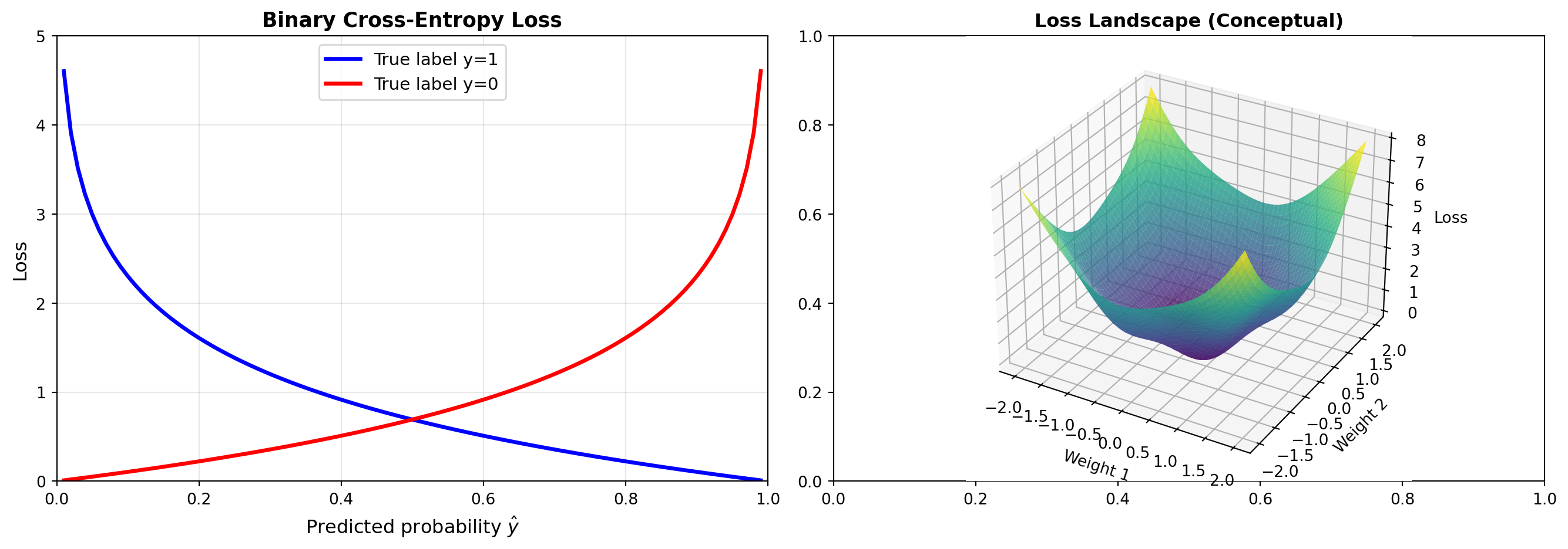
3.1 The Loss Function
For binary classification, we use Binary Cross-Entropy Loss:
Now let’s test our MLP on a more realistic dataset!
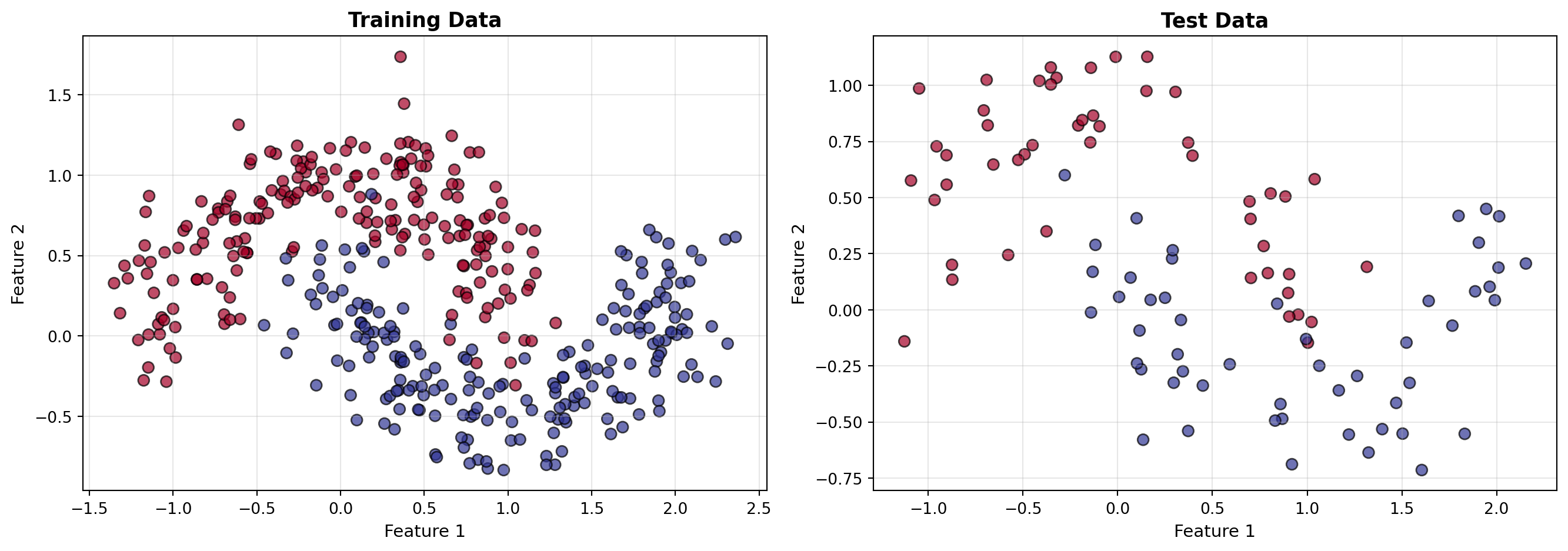
5.1 Creating the Dataset
We’ll create a synthetic 2D classification dataset (implementing everything from scratch!):
def make_moons_manual(n_samples=500, noise=0.2, seed=42):""" Create a moons dataset from scratch (no sklearn needed!) """ np.random.seed(seed) n_samples_per_moon = n_samples //2# First moon (upper) theta1 = np.linspace(0, np.pi, n_samples_per_moon) x1 = np.cos(theta1) y1 = np.sin(theta1)# Second moon (lower, shifted) theta2 = np.linspace(0, np.pi, n_samples_per_moon) x2 =1- np.cos(theta2) y2 =1- np.sin(theta2) -0.5# Combine X = np.vstack([ np.column_stack([x1, y1]), np.column_stack([x2, y2]) ])# Add noise X += np.random.normal(0, noise, X.shape)# Labels y = np.hstack([np.zeros(n_samples_per_moon), np.ones(n_samples_per_moon)]).astype(int)# Shuffle indices = np.random.permutation(n_samples)return X[indices], y[indices]def train_test_split_manual(X, y, test_size=0.2, seed=42):"""Split data into train and test sets""" np.random.seed(seed) n_samples =len(y) n_test =int(n_samples * test_size) indices = np.random.permutation(n_samples) test_idx, train_idx = indices[:n_test], indices[n_test:]return X[train_idx], X[test_idx], y[train_idx], y[test_idx]def standardize(X_train, X_test):"""Standardize features (zero mean, unit variance)""" mean = X_train.mean(axis=0) std = X_train.std(axis=0) X_train_scaled = (X_train - mean) / std X_test_scaled = (X_test - mean) / stdreturn X_train_scaled, X_test_scaled, mean, std# Create a moons datasetX, y = make_moons_manual(n_samples=500, noise=0.2, seed=42)# Split into train and testX_train, X_test, y_train, y_test = train_test_split_manual(X, y, test_size=0.2, seed=42)# Standardize featuresX_train_scaled, X_test_scaled, data_mean, data_std = standardize(X_train, X_test)# Transpose for our MLP (features × samples)X_train_T = X_train_scaled.TX_test_T = X_test_scaled.Ty_train_T = y_train.reshape(1, -1)y_test_T = y_test.reshape(1, -1)print("="*60)print("MOONS DATASET (Created from scratch!)")print("="*60)print(f"Training samples: {X_train_T.shape[1]}")print(f"Test samples: {X_test_T.shape[1]}")print(f"Features: {X_train_T.shape[0]}")print(f"Class distribution (train): {np.bincount(y_train)}")# Visualizefig, axes = plt.subplots(1, 2, figsize=(14, 5))# Training datascatter = axes[0].scatter(X_train[:, 0], X_train[:, 1], c=y_train, cmap='RdYlBu', edgecolors='black', alpha=0.7, s=50)axes[0].set_xlabel('Feature 1', fontsize=11)axes[0].set_ylabel('Feature 2', fontsize=11)axes[0].set_title('Training Data', fontsize=13, weight='bold')axes[0].grid(True, alpha=0.3)# Test dataaxes[1].scatter(X_test[:, 0], X_test[:, 1], c=y_test, cmap='RdYlBu', edgecolors='black', alpha=0.7, s=50)axes[1].set_xlabel('Feature 1', fontsize=11)axes[1].set_ylabel('Feature 2', fontsize=11)axes[1].set_title('Test Data', fontsize=13, weight='bold')axes[1].grid(True, alpha=0.3)plt.tight_layout()plt.show()
============================================================
MOONS DATASET (Created from scratch!)
============================================================
Training samples: 400
Test samples: 100
Features: 2
Class distribution (train): [201 199]
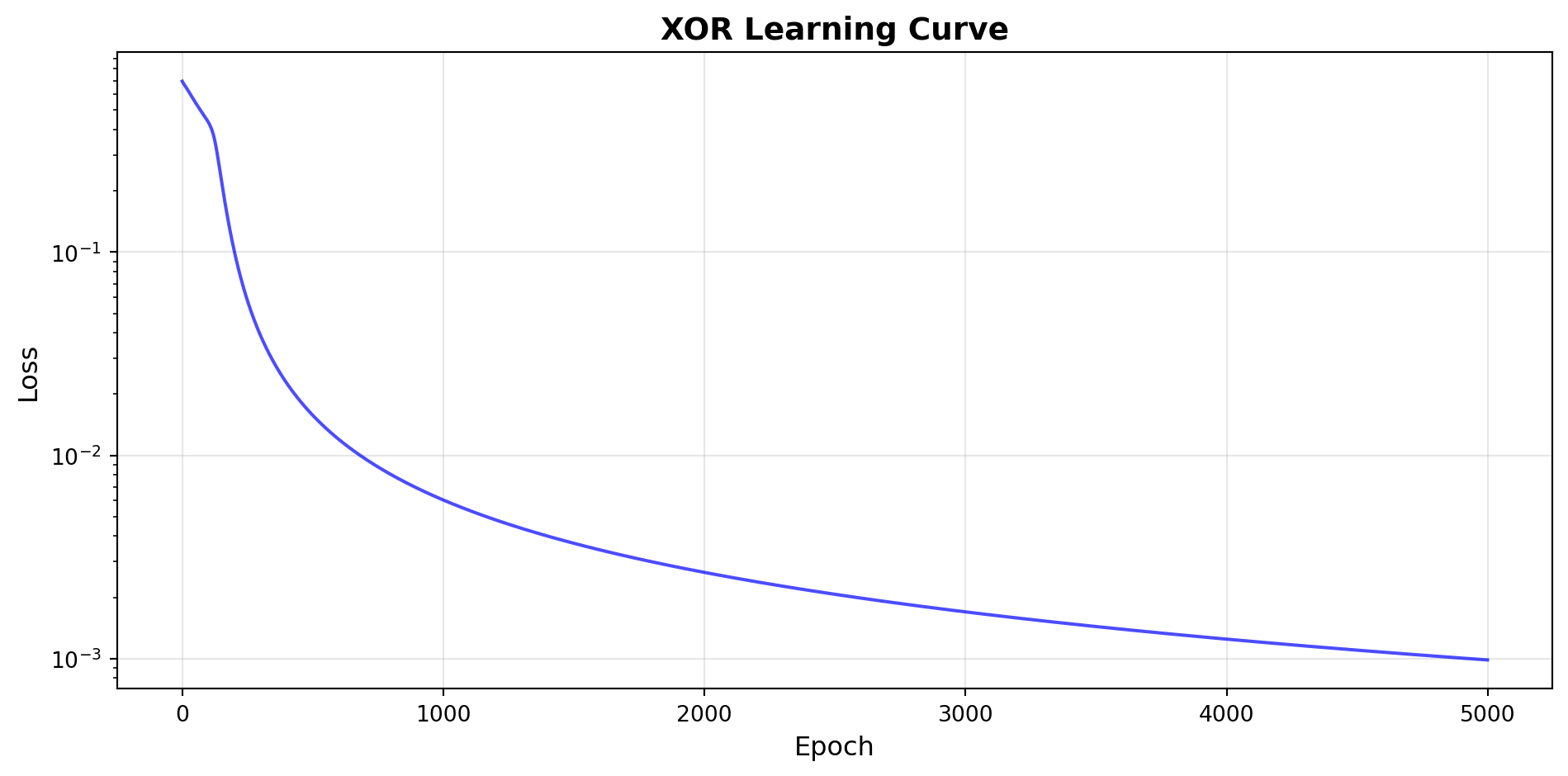
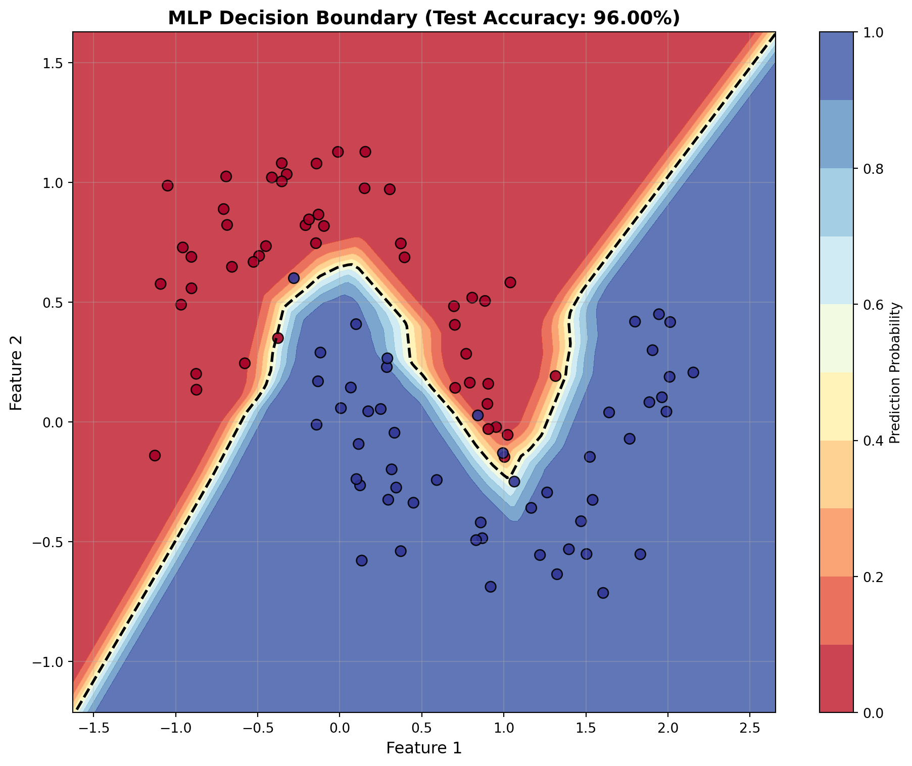
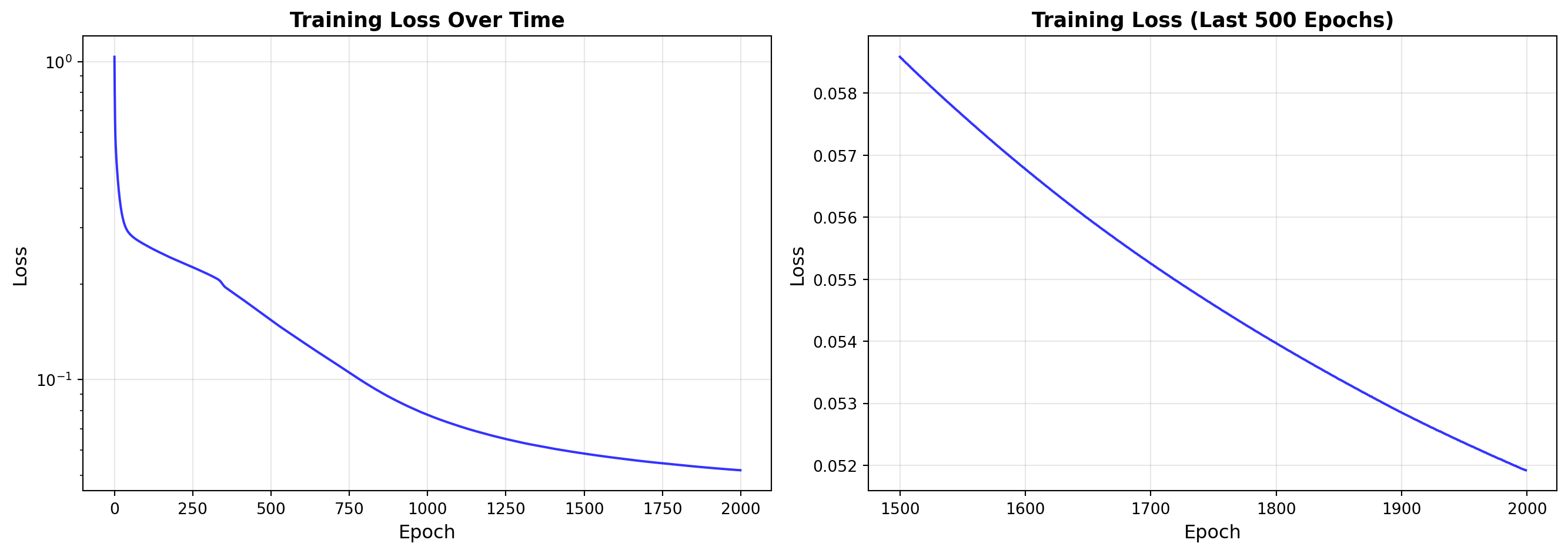
5.2 Training the MLP
# Create MLP with architecture suited for this problemmlp = MLP( layer_sizes=[2, 16, 8, 1], # 2 inputs → 16 → 8 → 1 output activations=['relu', 'relu', 'sigmoid'], learning_rate=0.1, seed=42)print(f"\n🏋️ Training on Moons Dataset...")print("-"*60)losses = mlp.train( X_train_T, y_train_T, epochs=2000, print_every=200, verbose=True)# Evaluate on test settest_accuracy = mlp.evaluate(X_test_T, y_test_T)train_accuracy = mlp.evaluate(X_train_T, y_train_T)print("\n"+"="*60)print("FINAL RESULTS")print("="*60)print(f"Training Accuracy: {train_accuracy:.2%}")print(f"Test Accuracy: {test_accuracy:.2%}")print("="*60)
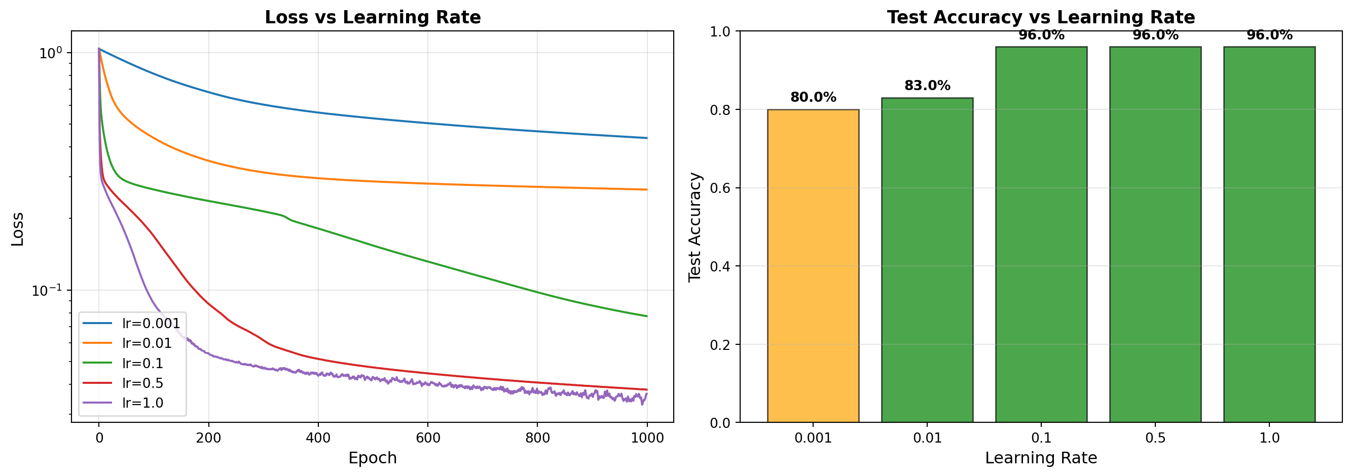
==================================================
LEARNING RATE COMPARISON
==================================================
lr = 0.001 → Test Accuracy: 80.00% ⚠️
lr =  0.01 → Test Accuracy: 83.00% ✅
lr =   0.1 → Test Accuracy: 96.00% ✅
lr =   0.5 → Test Accuracy: 96.00% ✅
lr =   1.0 → Test Accuracy: 96.00% ✅
==================================================
Part 7: Summary and Key Takeaways
7.1 What We Learned
Key Takeaways
Neural Network Basics:
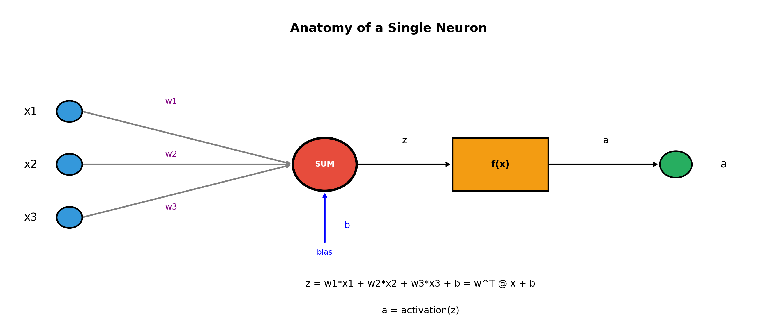
Neurons compute weighted sums + bias, then apply activation functions
Problem 5: Different Dataset Create a circles dataset (two concentric circles) from scratch and train the MLP on it. Compare results with the moons dataset.
Happy Learning! May your gradients always flow smoothly! 🚀
Questions or feedback? Feel free to reach out or open an issue on GitHub!