import pandas as pd
import numpy as np

# Check your pandas version
print(f"Pandas version: {pd.__version__}")
Pandas version: 2.0.3A hands-on journey through Python’s most powerful data analysis library
This tutorial will transform you from a pandas beginner into a confident data analyst. We’ll learn through fun, bite-sized examples using relatable datasets like student grades, coffee shop sales, and superhero statistics!
What makes this tutorial special?
Think of Pandas as a supercharged spreadsheet that lives inside Python. It can:
import pandas as pd
import numpy as np
# Check your pandas version
print(f"Pandas version: {pd.__version__}")Pandas version: 2.0.3Pandas has two main data structures. Think of them as building blocks:
A Series is like a labeled list. Every item has an index (label) and a value.
# Let's track daily temperatures for a week
temperatures = pd.Series(
    [22, 25, 23, 28, 30, 27, 24],
    index=['Mon', 'Tue', 'Wed', 'Thu', 'Fri', 'Sat', 'Sun'],
    name='Temperature (°C)'
)

print(temperatures)
print(f"\nHottest day: {temperatures.idxmax()} at {temperatures.max()}°C")
Mon 22
Tue 25
Wed 23
Thu 28
Fri 30
Sat 27
Sun 24
Name: Temperature (°C), dtype: int64
Hottest day: Fri at 30°CA DataFrame is a collection of Series that share the same index - essentially a table with rows and columns.
# Our first DataFrame: A tiny coffee shop!
coffee_shop = pd.DataFrame({
    'drink': ['Espresso', 'Latte', 'Cappuccino', 'Mocha', 'Americano'],
    'price': [2.50, 4.00, 3.75, 4.50, 3.00],
    'calories': [5, 190, 120, 290, 15],
    'has_milk': [False, True, True, True, False]
})

coffee_shop| drink | price | calories | has_milk | |
|---|---|---|---|---|
| 0 | Espresso | 2.50 | 5 | False |
| 1 | Latte | 4.00 | 190 | True |
| 2 | Cappuccino | 3.75 | 120 | True |
| 3 | Mocha | 4.50 | 290 | True |
| 4 | Americano | 3.00 | 15 | False |
You can create DataFrames from:
Using the coffee_shop DataFrame created above:
weekend_prices that increases all drink prices by 15%Hint: Use boolean filtering and remember that you can add rows with pd.concat()!
Before doing anything with data, always explore it first. Here’s your exploration toolkit:
# Let's create a more interesting dataset: Student exam scores
np.random.seed(42)  # For reproducibility

students = pd.DataFrame({
    'name': ['Alice', 'Bob', 'Charlie', 'Diana', 'Eve', 'Frank', 'Grace', 'Henry'],
    'age': [20, 21, 19, 22, 20, 23, 21, 20],
    'major': ['CS', 'Math', 'CS', 'Physics', 'Math', 'CS', 'Physics', 'Math'],
    'math_score': [85, 92, 78, 95, 88, 72, 91, 84],
    'python_score': [90, 85, 82, 88, 91, 95, 87, 79],
    'study_hours': [15, 20, 12, 25, 18, 10, 22, 14]
})

students| name | age | major | math_score | python_score | study_hours | |
|---|---|---|---|---|---|---|
| 0 | Alice | 20 | CS | 85 | 90 | 15 |
| 1 | Bob | 21 | Math | 92 | 85 | 20 |
| 2 | Charlie | 19 | CS | 78 | 82 | 12 |
| 3 | Diana | 22 | Physics | 95 | 88 | 25 |
| 4 | Eve | 20 | Math | 88 | 91 | 18 |
| 5 | Frank | 23 | CS | 72 | 95 | 10 |
| 6 | Grace | 21 | Physics | 91 | 87 | 22 |
| 7 | Henry | 20 | Math | 84 | 79 | 14 |
# Quick peek at first/last rows
print("=== First 3 rows ===")
print(students.head(3))
=== First 3 rows ===
name age major math_score python_score study_hours
0 Alice 20 CS 85 90 15
1 Bob 21 Math 92 85 20
2 Charlie 19 CS 78 82 12# Shape: (rows, columns)
print(f"\nDataset shape: {students.shape[0]} students, {students.shape[1]} attributes")
Dataset shape: 8 students, 6 attributes# Data types for each column
print("\n=== Column Data Types ===")
print(students.dtypes)
=== Column Data Types ===
name            object
age              int64
major           object
math_score       int64
python_score     int64
study_hours      int64
dtype: object
# Comprehensive info
print("\n=== DataFrame Info ===")
students.info()
=== DataFrame Info ===
<class 'pandas.core.frame.DataFrame'>
RangeIndex: 8 entries, 0 to 7
Data columns (total 6 columns):
 #   Column        Non-Null Count  Dtype
---  ------        --------------  -----
 0   name          8 non-null      object
 1   age           8 non-null      int64
 2   major         8 non-null      object
 3   math_score    8 non-null      int64
 4   python_score  8 non-null      int64
 5   study_hours   8 non-null      int64
dtypes: int64(4), object(2)
memory usage: 512.0+ bytes
# Statistical summary (only numeric columns by default)
print("\n=== Statistical Summary ===")
students.describe()
=== Statistical Summary ===| age | math_score | python_score | study_hours | |
|---|---|---|---|---|
| count | 8.00000 | 8.000000 | 8.000000 | 8.000000 |
| mean | 20.75000 | 85.625000 | 87.125000 | 17.000000 |
| std | 1.28174 | 7.652031 | 5.111262 | 5.154748 |
| min | 19.00000 | 72.000000 | 79.000000 | 10.000000 |
| 25% | 20.00000 | 82.500000 | 84.250000 | 13.500000 |
| 50% | 20.50000 | 86.500000 | 87.500000 | 16.500000 |
| 75% | 21.25000 | 91.250000 | 90.250000 | 20.500000 |
| max | 23.00000 | 95.000000 | 95.000000 | 25.000000 |
If you want to see statistics for ALL columns including text, use:
df.describe(include='all')Using the students DataFrame:
math_score and python_score (in absolute terms). Who is it and what’s the difference?.corr()Hint: abs() works with pandas Series, and you can use idxmax() to find the index of the maximum value!
This is where pandas really shines. Let’s master the art of data selection!
[]# Single column → Returns a Series
names = students['name']
print(type(names))
print(names)<class 'pandas.core.series.Series'>
0 Alice
1 Bob
2 Charlie
3 Diana
4 Eve
5 Frank
6 Grace
7 Henry
Name: name, dtype: object# Multiple columns → Returns a DataFrame
# Note the DOUBLE brackets!
scores = students[['name', 'math_score', 'python_score']]
scores| name | math_score | python_score | |
|---|---|---|---|
| 0 | Alice | 85 | 90 |
| 1 | Bob | 92 | 85 |
| 2 | Charlie | 78 | 82 |
| 3 | Diana | 95 | 88 |
| 4 | Eve | 88 | 91 |
| 5 | Frank | 72 | 95 |
| 6 | Grace | 91 | 87 |
| 7 | Henry | 84 | 79 |
# Row slicing (by position)
first_three = students[:3]
first_three| name | age | major | math_score | python_score | study_hours | |
|---|---|---|---|---|---|---|
| 0 | Alice | 20 | CS | 85 | 90 | 15 |
| 1 | Bob | 21 | Math | 92 | 85 | 20 |
| 2 | Charlie | 19 | CS | 78 | 82 | 12 |
.loc[].loc[] uses labels (names) to select data. Think “loc = label location”
# Select row by index label
students_indexed = students.set_index('name')
print(students_indexed.loc['Alice'])
age 20
major CS
math_score 85
python_score 90
study_hours 15
Name: Alice, dtype: object# Select specific rows and columns
students_indexed.loc[['Alice', 'Bob', 'Eve'], ['major', 'math_score']]| major | math_score | |
|---|---|---|
| name | ||
| Alice | CS | 85 |
| Bob | Math | 92 |
| Eve | Math | 88 |
# Slice with labels (INCLUSIVE on both ends!)
students_indexed.loc['Bob':'Eve', 'age':'python_score']| age | major | math_score | python_score | |
|---|---|---|---|---|
| name | ||||
| Bob | 21 | Math | 92 | 85 |
| Charlie | 19 | CS | 78 | 82 |
| Diana | 22 | Physics | 95 | 88 |
| Eve | 20 | Math | 88 | 91 |
.iloc[].iloc[] uses integer positions. Think “integer location”
# Select by row position
print("Row at position 0:")
print(students.iloc[0])
Row at position 0:
name Alice
age 20
major CS
math_score 85
python_score 90
study_hours 15
Name: 0, dtype: object# Select by row and column positions
# Rows 0-2 (exclusive), Columns 0-3 (exclusive)
students.iloc[0:3, 0:4]| name | age | major | math_score | |
|---|---|---|---|---|
| 0 | Alice | 20 | CS | 85 |
| 1 | Bob | 21 | Math | 92 |
| 2 | Charlie | 19 | CS | 78 |
# Cherry-pick specific positions
students.iloc[[0, 2, 4], [0, 3, 4]] # Rows 0,2,4 and columns 0,3,4| name | math_score | python_score | |
|---|---|---|---|
| 0 | Alice | 85 | 90 |
| 2 | Charlie | 78 | 82 |
| 4 | Eve | 88 | 91 |
| Feature | .loc[] |
.iloc[] |
|---|---|---|
| Uses | Labels/names | Integer positions |
| End of slice | Inclusive | Exclusive |
| Example | df.loc['a':'c'] includes ‘c’ |
df.iloc[0:3] excludes index 3 |
This is where data analysis gets exciting!
# Students who scored above 85 in math
high_math = students[students['math_score'] > 85]
high_math| name | age | major | math_score | python_score | study_hours | |
|---|---|---|---|---|---|---|
| 1 | Bob | 21 | Math | 92 | 85 | 20 |
| 3 | Diana | 22 | Physics | 95 | 88 | 25 |
| 4 | Eve | 20 | Math | 88 | 91 | 18 |
| 6 | Grace | 21 | Physics | 91 | 87 | 22 |
# Multiple conditions: Use & (and), | (or)
# IMPORTANT: Wrap each condition in parentheses!
cs_high_performers = students[
    (students['major'] == 'CS') &
    (students['python_score'] >= 85)
]
cs_high_performers| name | age | major | math_score | python_score | study_hours | |
|---|---|---|---|---|---|---|
| 0 | Alice | 20 | CS | 85 | 90 | 15 |
| 5 | Frank | 23 | CS | 72 | 95 | 10 |
# Using isin() for multiple values
math_or_physics = students[students['major'].isin(['Math', 'Physics'])]
math_or_physics| name | age | major | math_score | python_score | study_hours | |
|---|---|---|---|---|---|---|
| 1 | Bob | 21 | Math | 92 | 85 | 20 |
| 3 | Diana | 22 | Physics | 95 | 88 | 25 |
| 4 | Eve | 20 | Math | 88 | 91 | 18 |
| 6 | Grace | 21 | Physics | 91 | 87 | 22 |
| 7 | Henry | 20 | Math | 84 | 79 | 14 |
# Combining everything: Complex query
# "Find CS or Math students aged 20-21 who study more than 12 hours"
result = students[
    (students['major'].isin(['CS', 'Math'])) &
    (students['age'].between(20, 21)) &
    (students['study_hours'] > 12)
]
result| name | age | major | math_score | python_score | study_hours | |
|---|---|---|---|---|---|---|
| 0 | Alice | 20 | CS | 85 | 90 | 15 |
| 1 | Bob | 21 | Math | 92 | 85 | 20 |
| 4 | Eve | 20 | Math | 88 | 91 | 18 |
| 7 | Henry | 20 | Math | 84 | 79 | 14 |
The university wants to award scholarships! Using the students DataFrame, find all students who meet ALL of these criteria:
How many students qualify? What are their names?
Bonus: Use the .query() method instead of boolean indexing to solve the same problem!
# Simple calculation: Total score
students['total_score'] = students['math_score'] + students['python_score']

# Average score
students['avg_score'] = students['total_score'] / 2

# Score per study hour (efficiency metric!)
students['score_per_hour'] = (students['avg_score'] / students['study_hours']).round(2)

students[['name', 'avg_score', 'study_hours', 'score_per_hour']]| name | avg_score | study_hours | score_per_hour | |
|---|---|---|---|---|
| 0 | Alice | 87.5 | 15 | 5.83 |
| 1 | Bob | 88.5 | 20 | 4.42 |
| 2 | Charlie | 80.0 | 12 | 6.67 |
| 3 | Diana | 91.5 | 25 | 3.66 |
| 4 | Eve | 89.5 | 18 | 4.97 |
| 5 | Frank | 83.5 | 10 | 8.35 |
| 6 | Grace | 89.0 | 22 | 4.05 |
| 7 | Henry | 81.5 | 14 | 5.82 |
# Method 1: List comprehension
students['grade'] = ['A' if x >= 85 else 'B' if x >= 75 else 'C'
                     for x in students['avg_score']]

# Method 2: np.where (faster for large datasets)
students['passed'] = np.where(students['avg_score'] >= 70, 'Yes', 'No')

# Method 3: apply() with custom function
def categorize_study(hours):
    if hours >= 20:
        return 'Heavy Studier'
    elif hours >= 15:
        return 'Moderate'
    else:
        return 'Light Studier'

students['study_category'] = students['study_hours'].apply(categorize_study)

students[['name', 'grade', 'passed', 'study_category']]| name | grade | passed | study_category | |
|---|---|---|---|---|
| 0 | Alice | A | Yes | Moderate |
| 1 | Bob | A | Yes | Heavy Studier |
| 2 | Charlie | B | Yes | Light Studier |
| 3 | Diana | A | Yes | Heavy Studier |
| 4 | Eve | A | Yes | Moderate |
| 5 | Frank | B | Yes | Light Studier |
| 6 | Grace | A | Yes | Heavy Studier |
| 7 | Henry | B | Yes | Light Studier |
# Create a copy to experiment
df = students.copy()

# Curve everyone's math score by 5 points
df['math_score'] = df['math_score'] + 5

# Cap at 100
df['math_score'] = df['math_score'].clip(upper=100)

# Modify specific cells using .loc
df.loc[df['name'] == 'Frank', 'study_hours'] = 15  # Frank decided to study more!

df[['name', 'math_score', 'study_hours']].head()| name | math_score | study_hours | |
|---|---|---|---|
| 0 | Alice | 90 | 15 |
| 1 | Bob | 97 | 20 |
| 2 | Charlie | 83 | 12 |
| 3 | Diana | 100 | 25 |
| 4 | Eve | 93 | 18 |
# BAD: Unpredictable behavior!
df[df['age'] > 20]['grade'] = 'A+'  # May not work!

# GOOD: Use .loc for assignment
df.loc[df['age'] > 20, 'grade'] = 'A+'The professor wants to apply a grading curve to the students:
curved_math that adds points to each student’s math score so that the class average becomes exactly 85performance_tier column that labels students as:
np.select() (look it up!) as an alternative to nested if-else for creating the performance_tierHint: Use .quantile() to find percentile boundaries!
# Reload fresh data
students = pd.DataFrame({
    'name': ['Alice', 'Bob', 'Charlie', 'Diana', 'Eve', 'Frank', 'Grace', 'Henry'],
    'age': [20, 21, 19, 22, 20, 23, 21, 20],
    'major': ['CS', 'Math', 'CS', 'Physics', 'Math', 'CS', 'Physics', 'Math'],
    'math_score': [85, 92, 78, 95, 88, 72, 91, 84],
    'python_score': [90, 85, 82, 88, 91, 95, 87, 79]
})

print("=== Individual Statistics ===")
print(f"Average math score: {students['math_score'].mean():.2f}")
print(f"Median python score: {students['python_score'].median():.2f}")
print(f"Std deviation of ages: {students['age'].std():.2f}")
print(f"Youngest student: {students['age'].min()} years old")
print(f"Highest math score: {students['math_score'].max()}")
=== Individual Statistics ===
Average math score: 85.62
Median python score: 87.50
Std deviation of ages: 1.28
Youngest student: 19 years old
Highest math score: 95GroupBy is the most important concept for data analysis. It works in three steps:
# Average scores by major
students.groupby('major')[['math_score', 'python_score']].mean()| math_score | python_score | |
|---|---|---|
| major | ||
| CS | 78.333333 | 89.0 |
| Math | 88.000000 | 85.0 |
| Physics | 93.000000 | 87.5 |
# Multiple aggregations at once
students.groupby('major').agg({
    'math_score': ['mean', 'max', 'min'],
    'python_score': ['mean', 'std'],
    'name': 'count'  # Count students per major
})| math_score | python_score | name | ||||
|---|---|---|---|---|---|---|
| mean | max | min | mean | std | count | |
| major | ||||||
| CS | 78.333333 | 85 | 72 | 89.0 | 6.557439 | 3 |
| Math | 88.000000 | 92 | 84 | 85.0 | 6.000000 | 3 |
| Physics | 93.000000 | 95 | 91 | 87.5 | 0.707107 | 2 |
# Named aggregations (cleaner output!)
summary = students.groupby('major').agg(
    avg_math=('math_score', 'mean'),
    avg_python=('python_score', 'mean'),
    student_count=('name', 'count'),
    youngest=('age', 'min'),
    oldest=('age', 'max')
).round(2)

summary| avg_math | avg_python | student_count | youngest | oldest | |
|---|---|---|---|---|---|
| major | |||||
| CS | 78.33 | 89.0 | 3 | 19 | 23 |
| Math | 88.00 | 85.0 | 3 | 20 | 21 |
| Physics | 93.00 | 87.5 | 2 | 21 | 22 |
# Group by multiple columns
students.groupby(['major', 'age'])['math_score'].mean()
major age
CS 19 78.0
20 85.0
23 72.0
Math 20 86.0
21 92.0
Physics 21 91.0
22 95.0
Name: math_score, dtype: float64# How many students in each major?
print(students['major'].value_counts())major
CS 3
Math 3
Physics 2
Name: count, dtype: int64# As percentages
print("\nPercentage breakdown:")
print(students['major'].value_counts(normalize=True).mul(100).round(1))
Percentage breakdown:
major
CS         37.5
Math       37.5
Physics    25.0
Name: proportion, dtype: float64The Dean wants a comprehensive department report! Create a summary table that shows for each major:
Challenge: Use .transform() to add a column showing how each student’s math score compares to their major’s average (as a difference: “above/below average by X points”)
Hint: For finding the top performer name per group, you might need to use .apply() with a custom function!
Real-world data is messy. Let’s learn to deal with it!
# Create dataset with missing values
messy_data = pd.DataFrame({
    'product': ['Apple', 'Banana', 'Cherry', 'Date', 'Elderberry'],
    'price': [1.20, np.nan, 2.50, 1.80, np.nan],
    'quantity': [100, 150, np.nan, 200, 80],
    'supplier': ['Farm A', None, 'Farm B', 'Farm A', 'Farm C']
})

messy_data| product | price | quantity | supplier | |
|---|---|---|---|---|
| 0 | Apple | 1.2 | 100.0 | Farm A |
| 1 | Banana | NaN | 150.0 | None |
| 2 | Cherry | 2.5 | NaN | Farm B |
| 3 | Date | 1.8 | 200.0 | Farm A |
| 4 | Elderberry | NaN | 80.0 | Farm C |
# Check for missing values
print("Missing values per column:")
print(messy_data.isna().sum())
Missing values per column:
product 0
price 2
quantity 1
supplier 1
dtype: int64# Percentage of missing values
print("\nPercentage missing:")
print((messy_data.isna().sum() / len(messy_data) * 100).round(1))
Percentage missing:
product      0.0
price       40.0
quantity    20.0
supplier    20.0
dtype: float64
# Find rows with ANY missing value
messy_data[messy_data.isna().any(axis=1)]| product | price | quantity | supplier | |
|---|---|---|---|---|
| 1 | Banana | NaN | 150.0 | None |
| 2 | Cherry | 2.5 | NaN | Farm B |
| 4 | Elderberry | NaN | 80.0 | Farm C |
# Option 1: Drop rows with missing values
clean_drop = messy_data.dropna()
print("After dropping missing rows:")
print(clean_drop)
After dropping missing rows:
product price quantity supplier
0 Apple 1.2 100.0 Farm A
3 Date 1.8 200.0 Farm A# Option 2: Fill with a specific value
filled_zero = messy_data.fillna(0)
print("\nAfter filling with 0:")
print(filled_zero)
After filling with 0:
      product  price  quantity supplier
0       Apple    1.2     100.0   Farm A
1      Banana    0.0     150.0        0
2      Cherry    2.5       0.0   Farm B
3        Date    1.8     200.0   Farm A
4  Elderberry    0.0      80.0   Farm C
# Option 3: Fill with column statistics (Smart filling!)
smart_fill = messy_data.copy()
smart_fill['price'] = smart_fill['price'].fillna(smart_fill['price'].mean())
smart_fill['quantity'] = smart_fill['quantity'].fillna(smart_fill['quantity'].median())
smart_fill['supplier'] = smart_fill['supplier'].fillna('Unknown')
print("\nAfter smart filling:")
print(smart_fill)
After smart filling:
      product     price  quantity supplier
0       Apple  1.200000     100.0   Farm A
1      Banana  1.833333     150.0  Unknown
2      Cherry  2.500000     125.0   Farm B
3        Date  1.800000     200.0   Farm A
4  Elderberry  1.833333      80.0   Farm C
# Option 4: Forward/backward fill (great for time series)
ts_data = pd.DataFrame({
'day': [1, 2, 3, 4, 5],
'temperature': [22, np.nan, np.nan, 25, 24]
})
print("Forward fill (use previous value):")
print(ts_data.ffill())Forward fill (use previous value):
day temperature
0 1 22.0
1 2 22.0
2 3 22.0
3 4 25.0
4 5 24.0You’re given this messy inventory data:
inventory = pd.DataFrame({
    'product': ['Widget', 'Gadget', 'Gizmo', 'Doohickey', 'Thingamajig'],
    'price': [10.0, np.nan, 25.0, np.nan, 15.0],
    'stock': [100, 50, np.nan, 75, np.nan],
    'category': ['Electronics', None, 'Electronics', 'Home', None],
    'last_sale': ['2024-01-15', '2024-01-10', np.nan, '2024-01-20', '2024-01-05']
})last_sale, forward-fill based on the sorted date orderBonus: Use .interpolate() to fill numeric missing values - how does this differ from using median?
# Class A students
class_a = pd.DataFrame({
    'name': ['Alice', 'Bob'],
    'score': [85, 92]
})

# Class B students
class_b = pd.DataFrame({
    'name': ['Charlie', 'Diana'],
    'score': [78, 95]
})

# Stack vertically (row-wise)
all_students = pd.concat([class_a, class_b], ignore_index=True)
all_students| name | score | |
|---|---|---|
| 0 | Alice | 85 |
| 1 | Bob | 92 |
| 2 | Charlie | 78 |
| 3 | Diana | 95 |
# Stack horizontally (column-wise)
scores_math = pd.DataFrame({'name': ['Alice', 'Bob'], 'math': [85, 92]})
scores_english = pd.DataFrame({'english': [90, 88]})

combined = pd.concat([scores_math, scores_english], axis=1)
combined| name | math | english | |
|---|---|---|---|
| 0 | Alice | 85 | 90 |
| 1 | Bob | 92 | 88 |
# Student info
students_info = pd.DataFrame({
    'student_id': [1, 2, 3, 4],
    'name': ['Alice', 'Bob', 'Charlie', 'Diana'],
    'major': ['CS', 'Math', 'CS', 'Physics']
})

# Course enrollment
enrollments = pd.DataFrame({
    'student_id': [1, 1, 2, 3, 5],  # Note: student 5 doesn't exist in students!
    'course': ['Python', 'Data Science', 'Calculus', 'Python', 'Chemistry'],
    'grade': ['A', 'A', 'B+', 'B', 'A-']
})

print("Students:")
print(students_info)
print("\nEnrollments:")
print(enrollments)
Students:
student_id name major
0 1 Alice CS
1 2 Bob Math
2 3 Charlie CS
3 4 Diana Physics
Enrollments:
student_id course grade
0 1 Python A
1 1 Data Science A
2 2 Calculus B+
3 3 Python B
4 5 Chemistry A-# Inner join: Only matching records
inner = pd.merge(students_info, enrollments, on='student_id', how='inner')
print("INNER JOIN (only matches):")
innerINNER JOIN (only matches):| student_id | name | major | course | grade | |
|---|---|---|---|---|---|
| 0 | 1 | Alice | CS | Python | A |
| 1 | 1 | Alice | CS | Data Science | A |
| 2 | 2 | Bob | Math | Calculus | B+ |
| 3 | 3 | Charlie | CS | Python | B |
# Left join: All from left, matching from right
left = pd.merge(students_info, enrollments, on='student_id', how='left')
print("LEFT JOIN (all students):")
left
LEFT JOIN (all students):| student_id | name | major | course | grade | |
|---|---|---|---|---|---|
| 0 | 1 | Alice | CS | Python | A |
| 1 | 1 | Alice | CS | Data Science | A |
| 2 | 2 | Bob | Math | Calculus | B+ |
| 3 | 3 | Charlie | CS | Python | B |
| 4 | 4 | Diana | Physics | NaN | NaN |
# Outer join: Everything from both
outer = pd.merge(students_info, enrollments, on='student_id', how='outer')
print("OUTER JOIN (everything):")
outer
OUTER JOIN (everything):| student_id | name | major | course | grade | |
|---|---|---|---|---|---|
| 0 | 1 | Alice | CS | Python | A |
| 1 | 1 | Alice | CS | Data Science | A |
| 2 | 2 | Bob | Math | Calculus | B+ |
| 3 | 3 | Charlie | CS | Python | B |
| 4 | 4 | Diana | Physics | NaN | NaN |
| 5 | 5 | NaN | NaN | Chemistry | A- |
| Join Type | What it keeps |
|---|---|
inner |
Only rows with matching keys in both tables |
left |
All rows from left table + matches from right |
right |
All rows from right table + matches from left |
outer |
All rows from both tables |
You’re building a music festival database with three tables:
artists = pd.DataFrame({
    'artist_id': [1, 2, 3, 4],
    'name': ['The Pandas', 'NumPy Knights', 'Data Frames', 'Index Error'],
    'genre': ['Rock', 'Electronic', 'Jazz', 'Pop']
})

performances = pd.DataFrame({
    'performance_id': [101, 102, 103, 104, 105],
    'artist_id': [1, 2, 1, 3, 5],  # Note: artist 5 doesn't exist!
    'stage': ['Main', 'Tent', 'Main', 'Acoustic', 'Main'],
    'time_slot': ['8PM', '9PM', '10PM', '7PM', '6PM']
})

ticket_sales = pd.DataFrame({
    'performance_id': [101, 101, 102, 103, 106],  # Note: performance 106 doesn't exist!
    'tickets_sold': [500, 300, 450, 600, 200]
})Hint: Think carefully about which join types to use for each question!
# Sales data in "long" format
sales_long = pd.DataFrame({
    'date': ['2024-01', '2024-01', '2024-02', '2024-02', '2024-03', '2024-03'],
    'product': ['Apple', 'Banana', 'Apple', 'Banana', 'Apple', 'Banana'],
    'sales': [100, 150, 120, 140, 130, 160]
})

print("Long format:")
print(sales_long)
Long format:
date product sales
0 2024-01 Apple 100
1 2024-01 Banana 150
2 2024-02 Apple 120
3 2024-02 Banana 140
4 2024-03 Apple 130
5 2024-03 Banana 160# Pivot to wide format
sales_wide = sales_long.pivot(index='date', columns='product', values='sales')
print("\nWide format (after pivot):")
sales_wide
Wide format (after pivot):| product | Apple | Banana |
|---|---|---|
| date | ||
| 2024-01 | 100 | 150 |
| 2024-02 | 120 | 140 |
| 2024-03 | 130 | 160 |
# Sales with multiple entries per date/product
sales_detailed = pd.DataFrame({
    'date': ['2024-01', '2024-01', '2024-01', '2024-02', '2024-02'],
    'product': ['Apple', 'Apple', 'Banana', 'Apple', 'Banana'],
    'store': ['Store A', 'Store B', 'Store A', 'Store A', 'Store B'],
    'sales': [50, 50, 150, 120, 140]
})

# Pivot table with aggregation
pivot_result = pd.pivot_table(
    sales_detailed,
    values='sales',
    index='date',
    columns='product',
    aggfunc='sum',
    margins=True  # Add row/column totals!
)

pivot_result| product | Apple | Banana | All |
|---|---|---|---|
| date | |||
| 2024-01 | 100 | 150 | 250 |
| 2024-02 | 120 | 140 | 260 |
| All | 220 | 290 | 510 |
# Wide format data
grades_wide = pd.DataFrame({
    'student': ['Alice', 'Bob', 'Charlie'],
    'Math': [85, 92, 78],
    'Science': [90, 85, 82],
    'English': [88, 91, 75]
})

print("Wide format:")
print(grades_wide)
Wide format:
student Math Science English
0 Alice 85 90 88
1 Bob 92 85 91
2 Charlie 78 82 75# Melt to long format
grades_long = pd.melt(
grades_wide,
id_vars=['student'], # Keep this column as-is
value_vars=['Math', 'Science', 'English'], # Melt these columns
var_name='subject', # Name for the melted column names
value_name='score' # Name for the melted values
)
print("\nLong format (after melt):")
grades_long
Long format (after melt):| student | subject | score | |
|---|---|---|---|
| 0 | Alice | Math | 85 |
| 1 | Bob | Math | 92 |
| 2 | Charlie | Math | 78 |
| 3 | Alice | Science | 90 |
| 4 | Bob | Science | 85 |
| 5 | Charlie | Science | 82 |
| 6 | Alice | English | 88 |
| 7 | Bob | English | 91 |
| 8 | Charlie | English | 75 |
You received survey results in an awkward format:
survey = pd.DataFrame({
    'respondent': ['Alice', 'Bob', 'Charlie'],
    'q1_satisfaction': [4, 5, 3],
    'q1_importance': [5, 4, 5],
    'q2_satisfaction': [3, 4, 4],
    'q2_importance': [4, 5, 3],
    'q3_satisfaction': [5, 3, 4],
    'q3_importance': [3, 4, 5]
})respondent, question, metric, score
question is q1/q2/q3 and metric is satisfaction/importanceHint: You might need to use string methods to split column names after melting!
Pandas was originally built for financial time series data - and it shows!
# Create a date range
dates = pd.date_range(start='2024-01-01', periods=10, freq='D')
print("Date range:")
print(dates)
Date range:
DatetimeIndex(['2024-01-01', '2024-01-02', '2024-01-03', '2024-01-04',
'2024-01-05', '2024-01-06', '2024-01-07', '2024-01-08',
'2024-01-09', '2024-01-10'],
dtype='datetime64[ns]', freq='D')# Time series of daily sales
daily_sales = pd.DataFrame({
'date': pd.date_range('2024-01-01', periods=30, freq='D'),
'sales': np.random.randint(100, 500, 30),
'customers': np.random.randint(20, 100, 30)
})
# Convert to datetime (if not already)
daily_sales['date'] = pd.to_datetime(daily_sales['date'])
daily_sales.head(10)| date | sales | customers | |
|---|---|---|---|
| 0 | 2024-01-01 | 202 | 68 |
| 1 | 2024-01-02 | 448 | 78 |
| 2 | 2024-01-03 | 370 | 61 |
| 3 | 2024-01-04 | 206 | 79 |
| 4 | 2024-01-05 | 171 | 99 |
| 5 | 2024-01-06 | 288 | 34 |
| 6 | 2024-01-07 | 120 | 81 |
| 7 | 2024-01-08 | 202 | 81 |
| 8 | 2024-01-09 | 221 | 66 |
| 9 | 2024-01-10 | 314 | 81 |
# Use .dt accessor for datetime properties
daily_sales['year'] = daily_sales['date'].dt.year
daily_sales['month'] = daily_sales['date'].dt.month
daily_sales['day'] = daily_sales['date'].dt.day
daily_sales['weekday'] = daily_sales['date'].dt.day_name()
daily_sales['is_weekend'] = daily_sales['date'].dt.dayofweek >= 5

daily_sales[['date', 'sales', 'weekday', 'is_weekend']].head(10)| date | sales | weekday | is_weekend | |
|---|---|---|---|---|
| 0 | 2024-01-01 | 202 | Monday | False |
| 1 | 2024-01-02 | 448 | Tuesday | False |
| 2 | 2024-01-03 | 370 | Wednesday | False |
| 3 | 2024-01-04 | 206 | Thursday | False |
| 4 | 2024-01-05 | 171 | Friday | False |
| 5 | 2024-01-06 | 288 | Saturday | True |
| 6 | 2024-01-07 | 120 | Sunday | True |
| 7 | 2024-01-08 | 202 | Monday | False |
| 8 | 2024-01-09 | 221 | Tuesday | False |
| 9 | 2024-01-10 | 314 | Wednesday | False |
# Set date as index for resampling
ts = daily_sales.set_index('date')

# Resample to weekly (sum of sales)
weekly_sales = ts['sales'].resample('W').sum()
print("Weekly sales totals:")
print(weekly_sales)
Weekly sales totals:
date
2024-01-07 1805
2024-01-14 2025
2024-01-21 2397
2024-01-28 2339
2024-02-04 687
Freq: W-SUN, Name: sales, dtype: int64# Multiple aggregations
weekly_summary = ts.resample('W').agg({
'sales': ['sum', 'mean'],
'customers': ['sum', 'mean']
})
weekly_summary| sales | customers | |||
|---|---|---|---|---|
| sum | mean | sum | mean | |
| date | ||||
| 2024-01-07 | 1805 | 257.857143 | 500 | 71.428571 |
| 2024-01-14 | 2025 | 289.285714 | 477 | 68.142857 |
| 2024-01-21 | 2397 | 342.428571 | 346 | 49.428571 |
| 2024-01-28 | 2339 | 334.142857 | 402 | 57.428571 |
| 2024-02-04 | 687 | 343.500000 | 90 | 45.000000 |
# Filter by date range using string indexing
ts_indexed = daily_sales.set_index('date')

# Select specific date range
mid_january = ts_indexed['2024-01-10':'2024-01-20']
mid_january| sales | customers | year | month | day | weekday | is_weekend | |
|---|---|---|---|---|---|---|---|
| date | |||||||
| 2024-01-10 | 314 | 81 | 2024 | 1 | 10 | Wednesday | False |
| 2024-01-11 | 430 | 70 | 2024 | 1 | 11 | Thursday | False |
| 2024-01-12 | 187 | 74 | 2024 | 1 | 12 | Friday | False |
| 2024-01-13 | 472 | 83 | 2024 | 1 | 13 | Saturday | True |
| 2024-01-14 | 199 | 22 | 2024 | 1 | 14 | Sunday | True |
| 2024-01-15 | 459 | 70 | 2024 | 1 | 15 | Monday | False |
| 2024-01-16 | 251 | 26 | 2024 | 1 | 16 | Tuesday | False |
| 2024-01-17 | 230 | 40 | 2024 | 1 | 17 | Wednesday | False |
| 2024-01-18 | 249 | 92 | 2024 | 1 | 18 | Thursday | False |
| 2024-01-19 | 408 | 58 | 2024 | 1 | 19 | Friday | False |
| 2024-01-20 | 357 | 37 | 2024 | 1 | 20 | Saturday | True |
Create a simulated stock price dataset and analyze it:
np.random.seed(42)
stock_data = pd.DataFrame({
    'date': pd.date_range('2023-01-01', periods=365, freq='D'),
    'price': 100 + np.random.randn(365).cumsum(),
    'volume': np.random.randint(1000000, 5000000, 365)
})
stock_data['date'] = pd.to_datetime(stock_data['date'])
stock_data = stock_data.set_index('date')Hint: Use .shift() for lagged values and .rolling() for moving averages!
The .str accessor gives you superpowers for text manipulation!
# Dataset with text data
employees = pd.DataFrame({
    'full_name': ['  John Smith  ', 'MARY JOHNSON', 'david williams', 'Sarah Brown-Davis'],
    'email': ['john.smith@company.com', 'mary.j@company.com', 'dwilliams@company.com', 'sarah.bd@company.com'],
    'department': ['Sales - North', 'Marketing - East', 'IT - Central', 'Sales - South']
})

employees| full_name | department | ||
|---|---|---|---|
| 0 | John Smith | john.smith@company.com | Sales - North |
| 1 | MARY JOHNSON | mary.j@company.com | Marketing - East |
| 2 | david williams | dwilliams@company.com | IT - Central |
| 3 | Sarah Brown-Davis | sarah.bd@company.com | Sales - South |
# Clean and standardize names
employees['clean_name'] = (employees['full_name']
    .str.strip()           # Remove leading/trailing whitespace
    .str.lower()           # Convert to lowercase
    .str.title()           # Capitalize first letter of each word
)

employees[['full_name', 'clean_name']]| full_name | clean_name | |
|---|---|---|
| 0 | John Smith | John Smith |
| 1 | MARY JOHNSON | Mary Johnson |
| 2 | david williams | David Williams |
| 3 | Sarah Brown-Davis | Sarah Brown-Davis |
# Extract username from email
employees['username'] = employees['email'].str.split('@').str[0]

# Extract department and region
employees['dept'] = employees['department'].str.split(' - ').str[0]
employees['region'] = employees['department'].str.split(' - ').str[1]

employees[['email', 'username', 'department', 'dept', 'region']]| username | department | dept | region | ||
|---|---|---|---|---|---|
| 0 | john.smith@company.com | john.smith | Sales - North | Sales | North |
| 1 | mary.j@company.com | mary.j | Marketing - East | Marketing | East |
| 2 | dwilliams@company.com | dwilliams | IT - Central | IT | Central |
| 3 | sarah.bd@company.com | sarah.bd | Sales - South | Sales | South |
# Find employees in Sales
sales_team = employees[employees['department'].str.contains('Sales')]
print("Sales team:")
print(sales_team['clean_name'].values)
Sales team:
['John Smith' 'Sarah Brown-Davis']# Find names starting with 'S'
s_names = employees[employees['clean_name'].str.startswith('S')]
print("\nNames starting with 'S':")
print(s_names['clean_name'].values)
Names starting with 'S':
['Sarah Brown-Davis']# Clean up department names
employees['department_clean'] = employees['department'].str.replace(' - ', ': ')
employees[['department', 'department_clean']]| department | department_clean | |
|---|---|---|
| 0 | Sales - North | Sales: North |
| 1 | Marketing - East | Marketing: East |
| 2 | IT - Central | IT: Central |
| 3 | Sales - South | Sales: South |
You’re analyzing web server logs stored in a DataFrame:
logs = pd.DataFrame({
    'raw_log': [
        '192.168.1.100 - - [15/Jan/2024:10:30:45] "GET /home HTTP/1.1" 200 1234',
        '10.0.0.55 - - [15/Jan/2024:10:31:02] "POST /api/users HTTP/1.1" 201 567',
        '192.168.1.100 - - [15/Jan/2024:10:31:15] "GET /about HTTP/1.1" 200 2345',
        '172.16.0.1 - - [15/Jan/2024:10:32:00] "GET /products HTTP/1.1" 404 123',
        '192.168.1.100 - - [15/Jan/2024:10:32:30] "DELETE /api/users/5 HTTP/1.1" 403 89'
    ]
})
Extract and create these columns from the raw log: 1. ip_address - the IP at the start 2. timestamp - parse the date/time into a proper datetime 3. method - GET, POST, DELETE, etc. 4. endpoint - the URL path (/home, /api/users, etc.) 5. status_code - as an integer 6. response_size - as an integer
Then answer: - Which IP made the most requests? - What percentage of requests were successful (status 200-299)? - Which endpoints returned errors (status >= 400)?
Hint: Use .str.extract() with regex groups or multiple .str.split() operations!
Pandas integrates seamlessly with Matplotlib for quick visualizations!
import matplotlib.pyplot as plt

# Sample data for visualization
np.random.seed(42)
viz_data = pd.DataFrame({
    'date': pd.date_range('2024-01-01', periods=100),
    'product_a': np.random.randn(100).cumsum() + 100,
    'product_b': np.random.randn(100).cumsum() + 100,
    'product_c': np.random.randn(100).cumsum() + 100
})
viz_data = viz_data.set_index('date')viz_data.plot(figsize=(10, 5), title='Product Sales Over Time')
plt.ylabel('Sales ($)')
plt.tight_layout()
plt.show()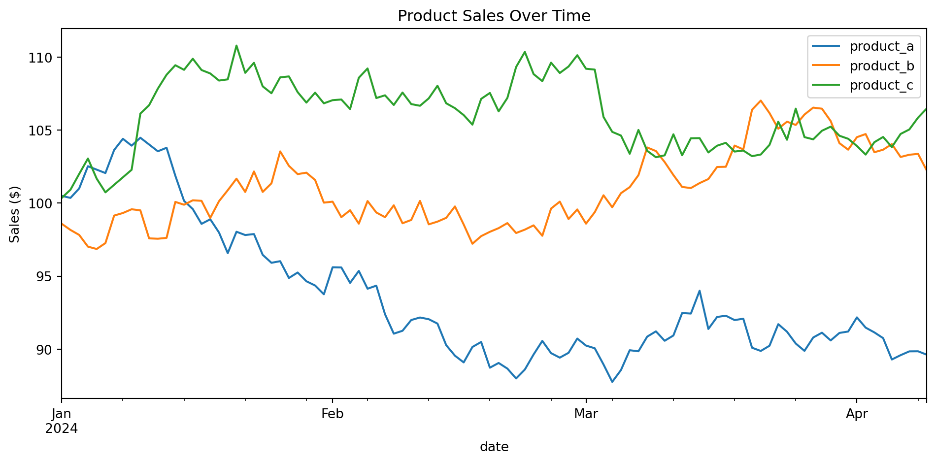
# Sample data
scores_by_major = pd.DataFrame({
    'Major': ['CS', 'Math', 'Physics', 'Chemistry'],
    'Avg Score': [87, 84, 91, 82]
}).set_index('Major')

scores_by_major.plot(kind='bar', figsize=(8, 5), color='steelblue', edgecolor='black')
plt.title('Average Scores by Major')
plt.ylabel('Score')
plt.xticks(rotation=45)
plt.tight_layout()
plt.show()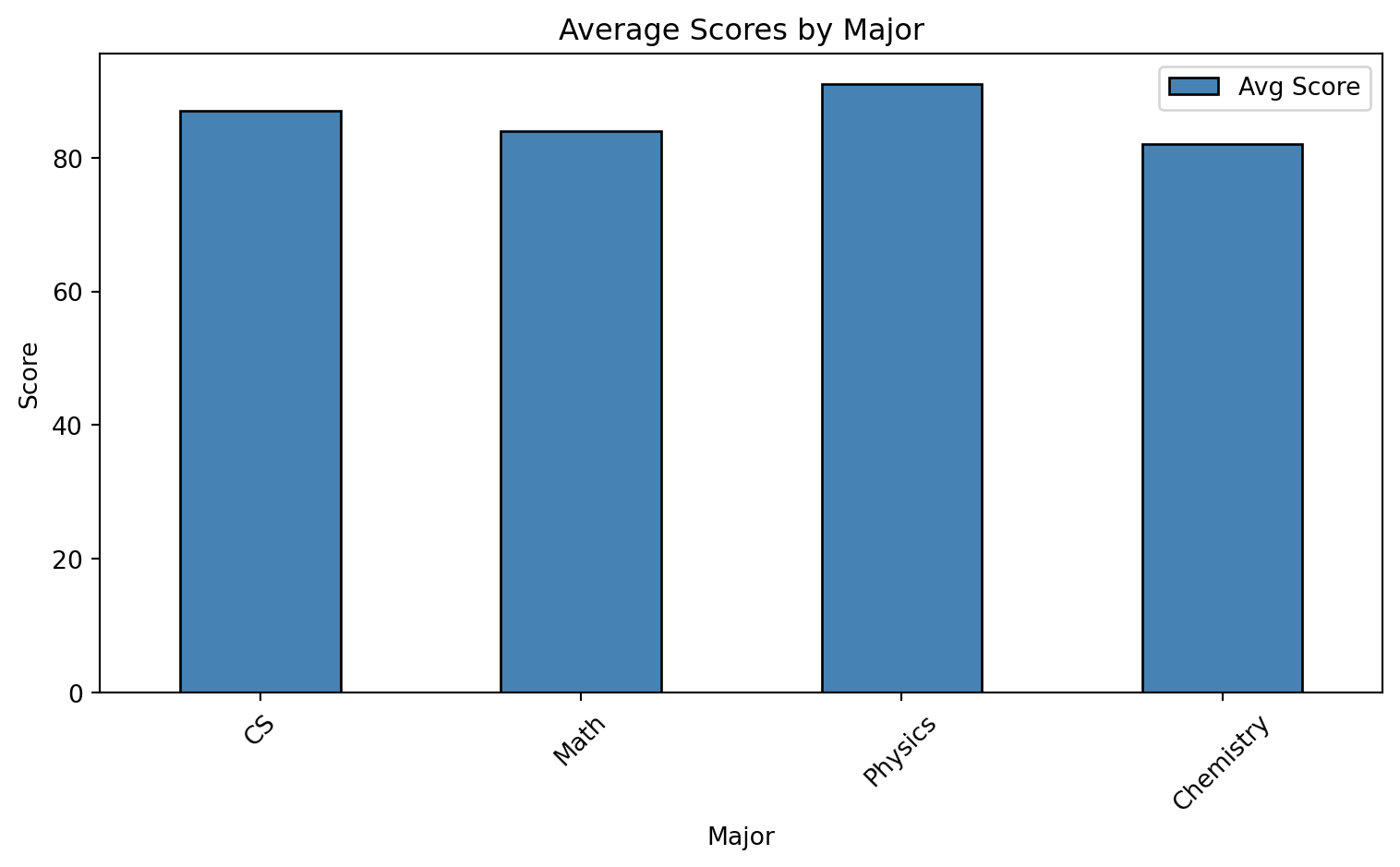
np.random.seed(42)
sales = pd.Series(np.random.normal(250, 50, 1000), name='Daily Sales')

sales.plot(kind='hist', bins=30, figsize=(8, 5), edgecolor='black', alpha=0.7)
plt.title('Distribution of Daily Sales')
plt.xlabel('Sales ($)')
plt.ylabel('Frequency')
plt.tight_layout()
plt.show()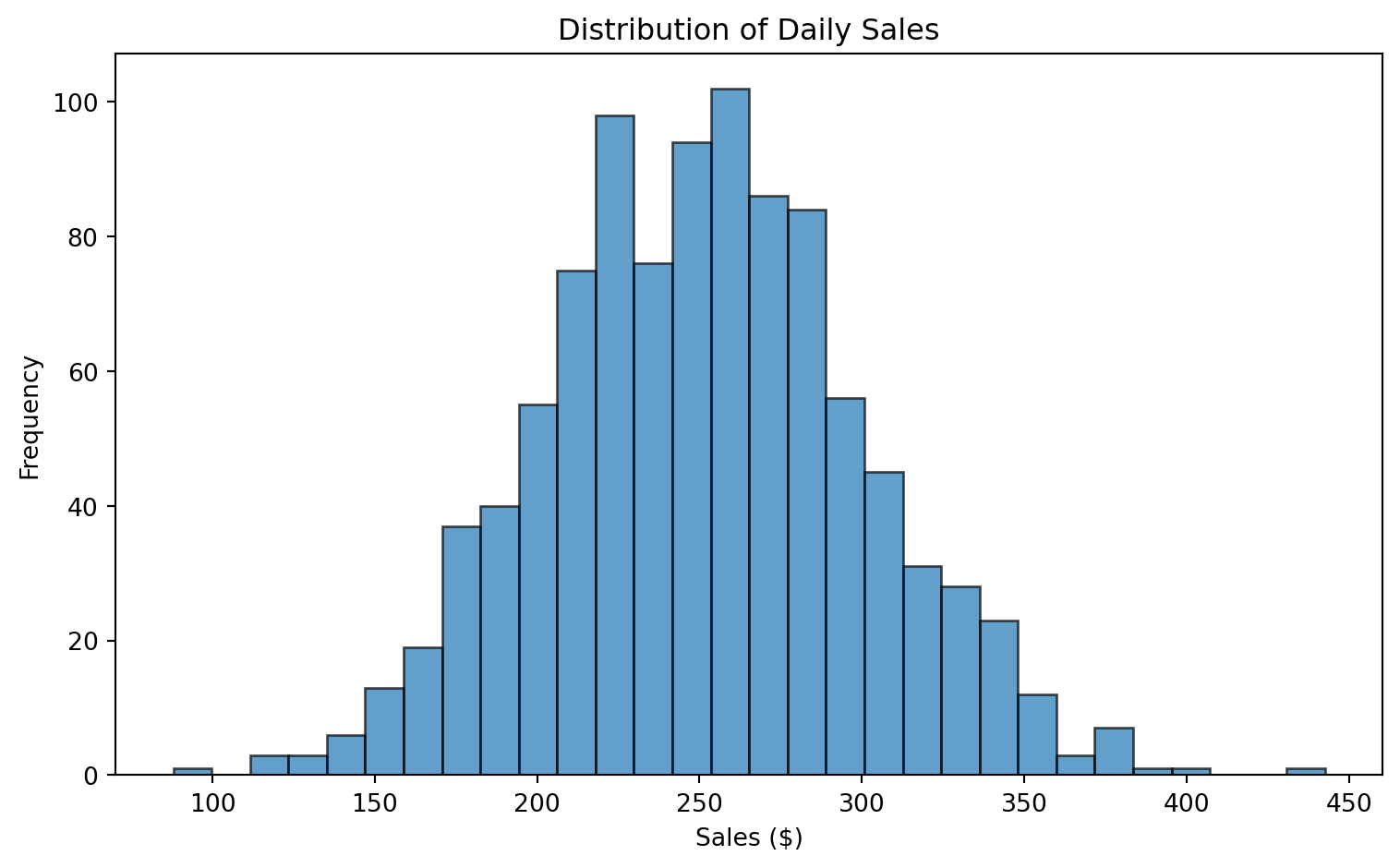
np.random.seed(42)
study_data = pd.DataFrame({
    'study_hours': np.random.uniform(1, 10, 50),
    'exam_score': lambda df: 50 + 5 * df['study_hours'] + np.random.normal(0, 5, 50)
})
study_data['exam_score'] = 50 + 5 * study_data['study_hours'] + np.random.normal(0, 5, 50)

study_data.plot(
    kind='scatter',
    x='study_hours',
    y='exam_score',
    figsize=(8, 5),
    alpha=0.6,
    c='steelblue',
    s=50
)
plt.title('Study Hours vs Exam Score')
plt.xlabel('Study Hours')
plt.ylabel('Exam Score')
plt.tight_layout()
plt.show()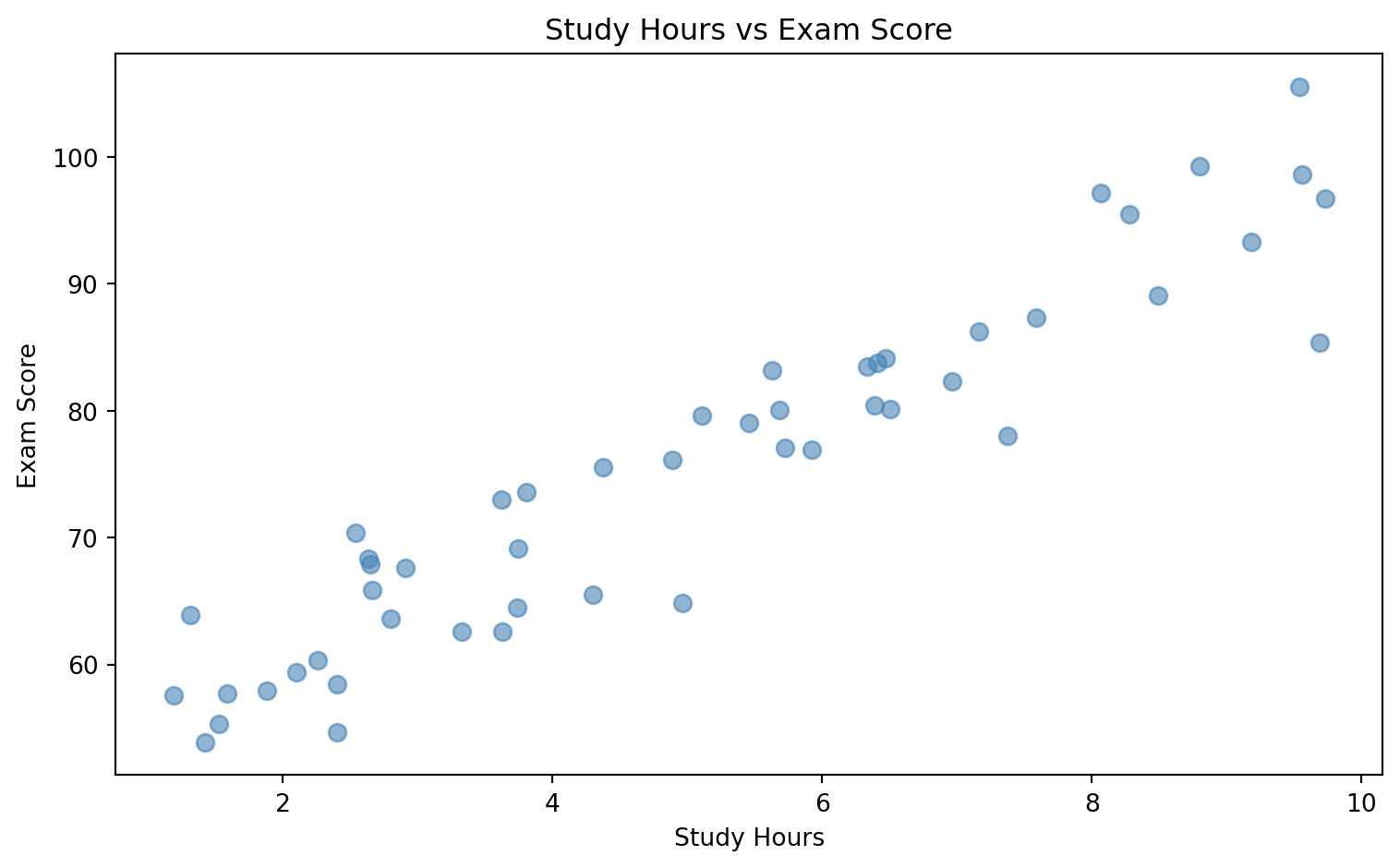
np.random.seed(42)
subject_scores = pd.DataFrame({
    'Math': np.random.normal(75, 10, 100),
    'Science': np.random.normal(80, 12, 100),
    'English': np.random.normal(78, 8, 100),
    'History': np.random.normal(72, 15, 100)
})

subject_scores.plot(kind='box', figsize=(8, 5))
plt.title('Score Distribution by Subject')
plt.ylabel('Score')
plt.tight_layout()
plt.show()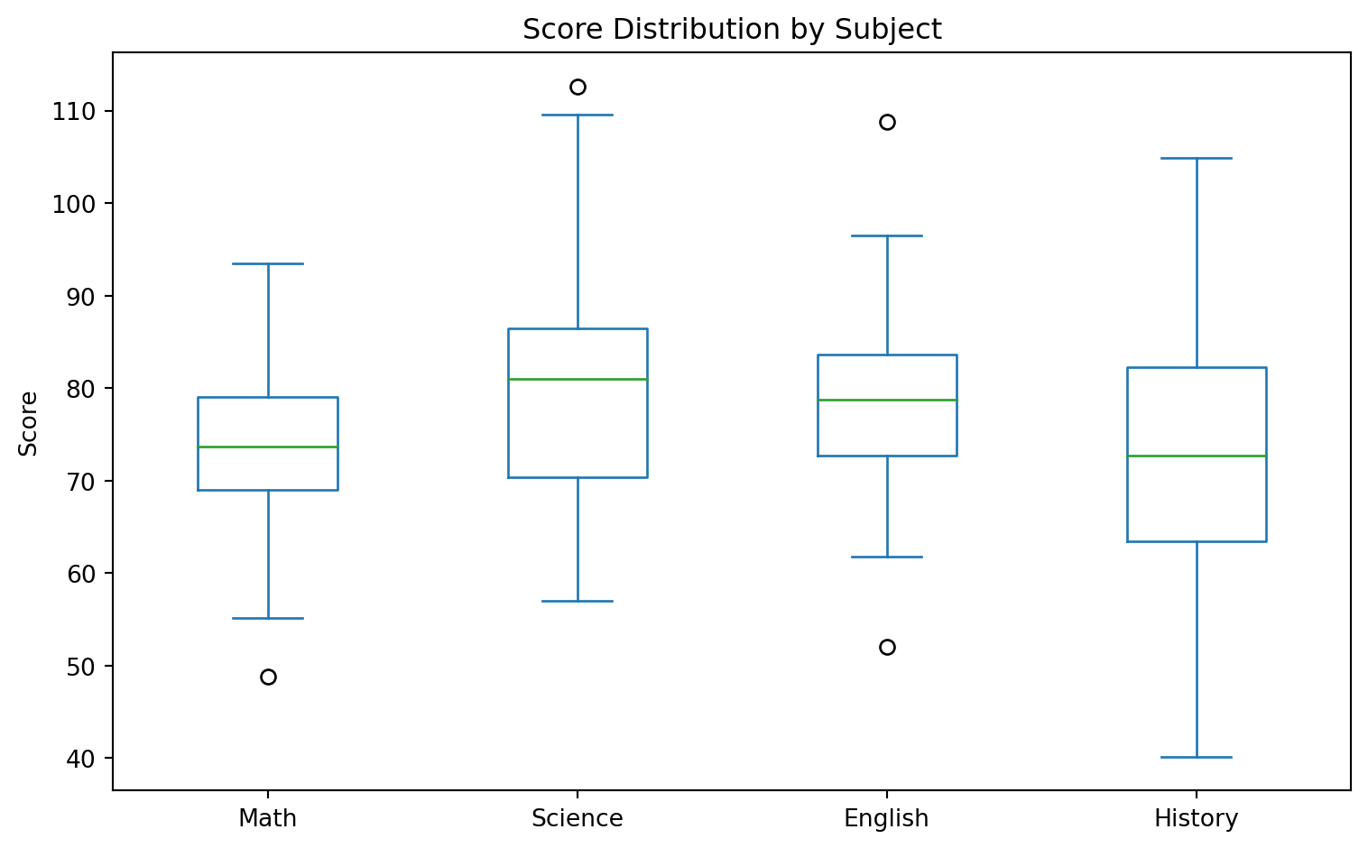
Create a mini sales dashboard! Using this data:
np.random.seed(42)
sales_data = pd.DataFrame({
    'date': pd.date_range('2024-01-01', periods=90, freq='D'),
    'region': np.random.choice(['North', 'South', 'East', 'West'], 90),
    'product': np.random.choice(['Laptop', 'Phone', 'Tablet', 'Watch'], 90),
    'units': np.random.randint(5, 50, 90),
    'revenue': np.random.uniform(500, 5000, 90).round(2)
})
Create a figure with 4 subplots (2x2 grid) showing: 1. Top-left: Line plot of daily total revenue over time 2. Top-right: Bar chart of total revenue by region 3. Bottom-left: Pie chart of units sold by product category 4. Bottom-right: Box plot comparing revenue distribution across regions
Bonus challenges: - Add a 7-day rolling average line to the daily revenue plot - Color the bars in the bar chart by whether they’re above or below average - Add proper titles, labels, and a main figure title
Hint: Use plt.subplots(2, 2, figsize=(12, 10)) and access individual axes with axes[0, 0], axes[0, 1], etc.
# Create sample data
sample_data = pd.DataFrame({
    'name': ['Alice', 'Bob', 'Charlie'],
    'age': [25, 30, 35],
    'city': ['NYC', 'LA', 'Chicago']
})

# Save to CSV
sample_data.to_csv('/tmp/sample.csv', index=False)
print("Saved to CSV!")

# Read back
loaded = pd.read_csv('/tmp/sample.csv')
loaded
Saved to CSV!| name | age | city | |
|---|---|---|---|
| 0 | Alice | 25 | NYC |
| 1 | Bob | 30 | LA |
| 2 | Charlie | 35 | Chicago |
# Save to Excel (requires openpyxl)
# sample_data.to_excel('sample.xlsx', sheet_name='People', index=False)

# Read from Excel
# df = pd.read_excel('sample.xlsx', sheet_name='People')# You can read directly from URLs!
# df = pd.read_csv('https://example.com/data.csv')# Common parameters for read_csv
df = pd.read_csv(
'data.csv',
sep=',', # Delimiter (comma is default)
header=0, # Row number for column names
names=['a', 'b'], # Custom column names
usecols=['a', 'b'], # Only read specific columns
dtype={'a': int}, # Specify data types
parse_dates=['date'], # Parse date columns
na_values=['NA', '?'], # Values to treat as NaN
nrows=1000, # Only read first N rows
skiprows=5 # Skip first N rows
)You’re building a data pipeline that needs to handle multiple file formats. Create the following workflow:
Create a sample dataset with 1000 rows containing: id, name, email, signup_date, plan (Free/Basic/Premium), monthly_spend
Save this data in three different formats:
Read each file back and verify they’re identical using .equals()
Create a function that:
signup_date parsed as datetimeplan as a categorical typemonthly_spend as floatBonus: Time how long it takes to read/write each format for a 100,000 row dataset. Which is fastest?
Hint: Use Path from pathlib to easily get file extensions, and try-except for format detection!
import time

# Create large dataset
large_df = pd.DataFrame({
    'a': np.random.randn(100000),
    'b': np.random.randn(100000)
})

# SLOW: Using apply with lambda
start = time.time()
result_slow = large_df.apply(lambda row: row['a'] + row['b'], axis=1)
slow_time = time.time() - start

# FAST: Vectorized operation
start = time.time()
result_fast = large_df['a'] + large_df['b']
fast_time = time.time() - start

print(f"Apply method: {slow_time:.4f} seconds")
print(f"Vectorized: {fast_time:.4f} seconds")
print(f"Speedup: {slow_time/fast_time:.1f}x faster!")
Apply method: 0.6021 seconds
Vectorized: 0.0007 seconds
Speedup: 915.0x faster!# Check memory usage
df = pd.DataFrame({
'integers': np.random.randint(0, 100, 10000),
'small_ints': np.random.randint(0, 10, 10000),
'categories': np.random.choice(['A', 'B', 'C'], 10000)
})
print("Before optimization:")
print(df.memory_usage(deep=True))Before optimization:
Index 128
integers 80000
small_ints 80000
categories 580000
dtype: int64# Optimize memory
df_optimized = df.copy()
df_optimized['integers'] = df_optimized['integers'].astype('int8')
df_optimized['small_ints'] = df_optimized['small_ints'].astype('int8')
df_optimized['categories'] = df_optimized['categories'].astype('category')
print("\nAfter optimization:")
print(df_optimized.memory_usage(deep=True))
After optimization:
Index           128
integers      10000
small_ints    10000
categories    10282
dtype: int64# BAD: Growing DataFrame in a loop
df = pd.DataFrame()
for i in range(1000):
df = pd.concat([df, pd.DataFrame({'a': [i]})]) # Slow!
# GOOD: Build list first, then create DataFrame
data = [{'a': i} for i in range(1000)]
df = pd.DataFrame(data) # Fast!# Clean and readable code with method chaining
result = (students
.query('math_score > 80')
.assign(total=lambda x: x['math_score'] + x['python_score'])
.sort_values('total', ascending=False)
.head(5)
[['name', 'total']]
)
result| name | total | |
|---|---|---|
| 3 | Diana | 183 |
| 4 | Eve | 179 |
| 6 | Grace | 178 |
| 1 | Bob | 177 |
| 0 | Alice | 175 |
You’ve inherited this slow code from a colleague. Your mission: make it at least 10x faster!
import time

# Generate test data
np.random.seed(42)
n = 100000
df = pd.DataFrame({
    'category': np.random.choice(['A', 'B', 'C', 'D', 'E'], n),
    'value1': np.random.randn(n),
    'value2': np.random.randn(n),
    'date': pd.date_range('2020-01-01', periods=n, freq='min')
})

# SLOW CODE - Optimize this!
start = time.time()

# Task 1: Calculate a weighted score for each row
results = []
for idx, row in df.iterrows():
    if row['category'] in ['A', 'B']:
        score = row['value1'] * 2 + row['value2']
    else:
        score = row['value1'] + row['value2'] * 2
    results.append(score)
df['score'] = results

# Task 2: Flag rows where score > category mean
category_means = {}
for cat in df['category'].unique():
    category_means[cat] = df[df['category'] == cat]['score'].mean()

flags = []
for idx, row in df.iterrows():
    if row['score'] > category_means[row['category']]:
        flags.append(True)
    else:
        flags.append(False)
df['above_avg'] = flags

# Task 3: Count above_avg per category per day
df['day'] = df['date'].apply(lambda x: x.date())
daily_counts = pd.DataFrame()
for day in df['day'].unique():
    for cat in df['category'].unique():
        subset = df[(df['day'] == day) & (df['category'] == cat)]
        count = subset['above_avg'].sum()
        daily_counts = pd.concat([daily_counts,
            pd.DataFrame({'day': [day], 'category': [cat], 'count': [count]})])

print(f"Slow version: {time.time() - start:.2f} seconds")
Rewrite all three tasks using vectorized pandas operations. Can you get it under 0.1 seconds?
Hint: Use np.where(), .transform(), .groupby(), and avoid iterrows() like the plague!
pd.DataFrame(dict)           # From dictionary
pd.DataFrame(list)           # From list of lists
pd.read_csv('file.csv')      # From CSV
pd.read_excel('file.xlsx') # From Exceldf.head() # First 5 rows
df.tail() # Last 5 rows
df.shape # (rows, columns)
df.info() # Column info
df.describe() # Statistics
df.dtypes # Data typesdf['col'] # Single column
df[['a', 'b']] # Multiple columns
df.loc[label] # By label
df.iloc[position] # By position
df[df['col'] > 5] # Boolean filterdf['new'] = values # Add column
df.drop('col', axis=1) # Remove column
df.rename(columns={}) # Rename columns
df.fillna(value) # Fill missing
df.dropna() # Drop missingdf.mean() # Average
df.sum() # Sum
df.groupby('col').mean() # Group + aggregate
df.value_counts() # Count categories
df.describe() # Summary statisticsdf.pivot() # Long to wide
df.melt() # Wide to long
pd.concat([df1, df2]) # Stack DataFrames
pd.merge(df1, df2) # Join DataFramesYou’ve learned:
Next steps:
Happy Data Analyzing!