The Perceiver Resampler: A Deep Dive into Visual Information Bottlenecks

Understanding how modern multimodal models compress visual information for language models

Deep Learning
Computer Vision
Multimodal Models
Attention Mechanisms
Author

Rishabh Mondal

Published

February 11, 2025

Welcome to the World of Multimodal Architecture!

Have you ever wondered how models like GPT-4V, Google Gemini, or DeepMind’s Flamingo can “see” images and have conversations about them? The secret lies in a beautiful architectural component called the Perceiver Resampler.

What you’ll learn in this blog:

  • Beginner: Why we need special architectures to bridge vision and language
  • Intermediate: The elegant solution using learned latent queries and cross-attention
  • Advanced: Temporal encodings, Fourier features, and implementation details
  • Expert: Complexity analysis, training strategies, and architectural decisions

Prerequisites: Basic understanding of neural networks and attention mechanisms. Don’t worry if you’re rusty—we’ll build up from the basics!


Executive Summary

TL;DR - The Core Idea

The Perceiver Resampler solves a critical problem in multimodal AI: vision encoders produce thousands of tokens, but language models need fixed-size inputs.

Key Innovation: Instead of processing visual features directly, use a small set of learned latent queries (typically 32-64 vectors) that act as “information extractors.” Through cross-attention, these latents query the visual features and compress them into a fixed-size representation.

Why it works: The latents learn to ask task-relevant questions—“Is there a dog?”, “What color is the car?”—and extract only the information needed.

Complexity: Reduces attention from \(O(M^2)\) (quadratic in input size) to \(O(MN + LN^2)\) (linear in input, where \(N \ll M\)).


Part 1: The Problem - Bridging Two Worlds

1.1 The Vision-Language Marriage

Modern AI has achieved something remarkable: we can now have natural conversations with AI about both text and images. But this marriage of vision and language faces a fundamental challenge:

The Scale Problem

Input Type Tokens Attention Computations
1 Image (ViT) ~578 patches ~334,000
8 Images (video) ~4,624 patches ~21,380,000
30 Frames (video) ~17,340 patches ~300,720,000
Text (512 tokens) 512 tokens ~262,000

The issue: Vision models produce a LOT of data. A single image might produce thousands of tokens. A video? That’s tens of thousands easily.

Language models expect fixed input sizes. GPT-style models process sequences where computational cost grows quadratically with sequence length.

The Quadratic Problem

In transformers, attention computes relationships between every pair of tokens. If you have \(n\) tokens, you need \(n^2\) computations.

\[ \text{Attention Complexity} = O(n^2 d) \]

Where \(n\) is sequence length and \(d\) is dimension. For 2,000 tokens at \(d=1024\): \[ 2,000^2 \times 1,024 = 4,096,000,000 \text{ operations!} \]

1.2 The Challenge: Variable Input, Fixed Output

We need a component that can:

  1. Accept variable-length visual input - 1 image, 8 images, 30 images… it should work with any number
  2. Produce fixed-size output - The language model needs a consistent representation
  3. Preserve important information - We can’t just randomly sample pixels!
  4. Be learnable - The model should figure out WHAT information matters

This is where the Perceiver Resampler enters the story.


Part 2: The Intuition - Building Understanding

2.1 The Library Analogy

Imagine you’re researching a topic and have access to a library with millions of books. You don’t have time to read everything, but you need enough information to write a comprehensive summary.

The Perceiver Resampler is like hiring a smart research assistant who:

  1. Has a set of pre-written research questions (learned latent queries)
  2. Searches through ALL the books (visual features)
  3. Extracts only the most relevant answers (cross-attention)
  4. Returns a fixed-size summary regardless of library size (fixed output)

The genius is that these “questions” aren’t fixed—they’re learned through training to extract exactly the information needed for the task!

2.2 The Information Bottleneck

Think of the Perceiver as a funnel:

Visual Input (Variable Size)
     |
     v
┌─────────────────┐
│  T × S tokens   │  -- Thousands of tokens
│   [M, d]        │
└────────┬────────┘
         │
         v  Cross-Attention (Learned Latents as Queries)
┌─────────────────┐
│  R latents      │  -- Fixed size (typically 32-64)
│   [N, d]        │
└────────┬────────┘
         │
         v  Deep Transformer Processing
┌─────────────────┐
│  Output         │  -- Rich, fixed-size representation
│   [N, d]        │
└─────────────────┘

Key insight: By forcing information through a narrow bottleneck, the model learns to preserve only the most task-relevant information.

2.3 Learned Latent Queries: The Secret Sauce

The key insight is that we don’t process visual features directly. Instead, we create a set of learned queries—vectors that start random but are trained to ask the right questions.

import numpy as np
import torch
import torch.nn as nn

# Imagine we have 64 "questions" our model can ask
# Each question is a vector of, say, 1024 dimensions
num_latents = 64
latent_dim = 1024

# At the start of training, these are random
learned_latents = torch.randn(num_latents, latent_dim)

print(f"Shape of learned latents: {learned_latents.shape}")
print(f"First few values of first latent: {learned_latents[0, :5].numpy()}")
# Output: torch.Size([64, 1024]) - 64 questions, each with 1024 dimensions
Shape of learned latents: torch.Size([64, 1024])
First few values of first latent: [ 0.10720182 -2.62119    -1.1030511  -0.73111475  0.9736447 ]

These “questions” aren’t text—they’re abstract vectors in a high-dimensional space. Through training, they learn to extract useful information from images.

Key Insight: Not Computed, But Learned!

The learned latents are NOT computed from the input images. They are:

  1. Initialized randomly at the start of training (like any neural network weights)
  2. Learned through backpropagation as the model trains on tasks
  3. Used as queries to extract information from any input

This is fundamentally different from computed features—they’re learnable parameters that specialize through gradient descent!


Part 3: Cross-Attention - The Mechanism

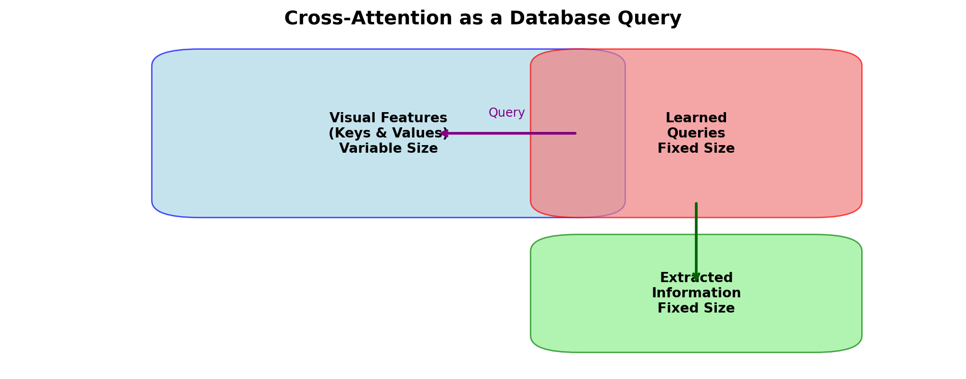
3.1 Understanding Cross-Attention

Before diving deeper, let’s understand cross-attention, the mechanism that powers the Perceiver Resampler.

Standard Self-Attention: Each token attends to every other token in the SAME sequence. \[ \text{Self-Attention}(X) = \text{softmax}\left(\frac{XW_Q (XW_K)^T}{\sqrt{d_k}}\right) XW_V \]

Cross-Attention: Tokens from one sequence attend to tokens from a DIFFERENT sequence. \[ \text{Cross-Attention}(Q, K, V) = \text{softmax}\left(\frac{QK^T}{\sqrt{d_k}}\right) V \]

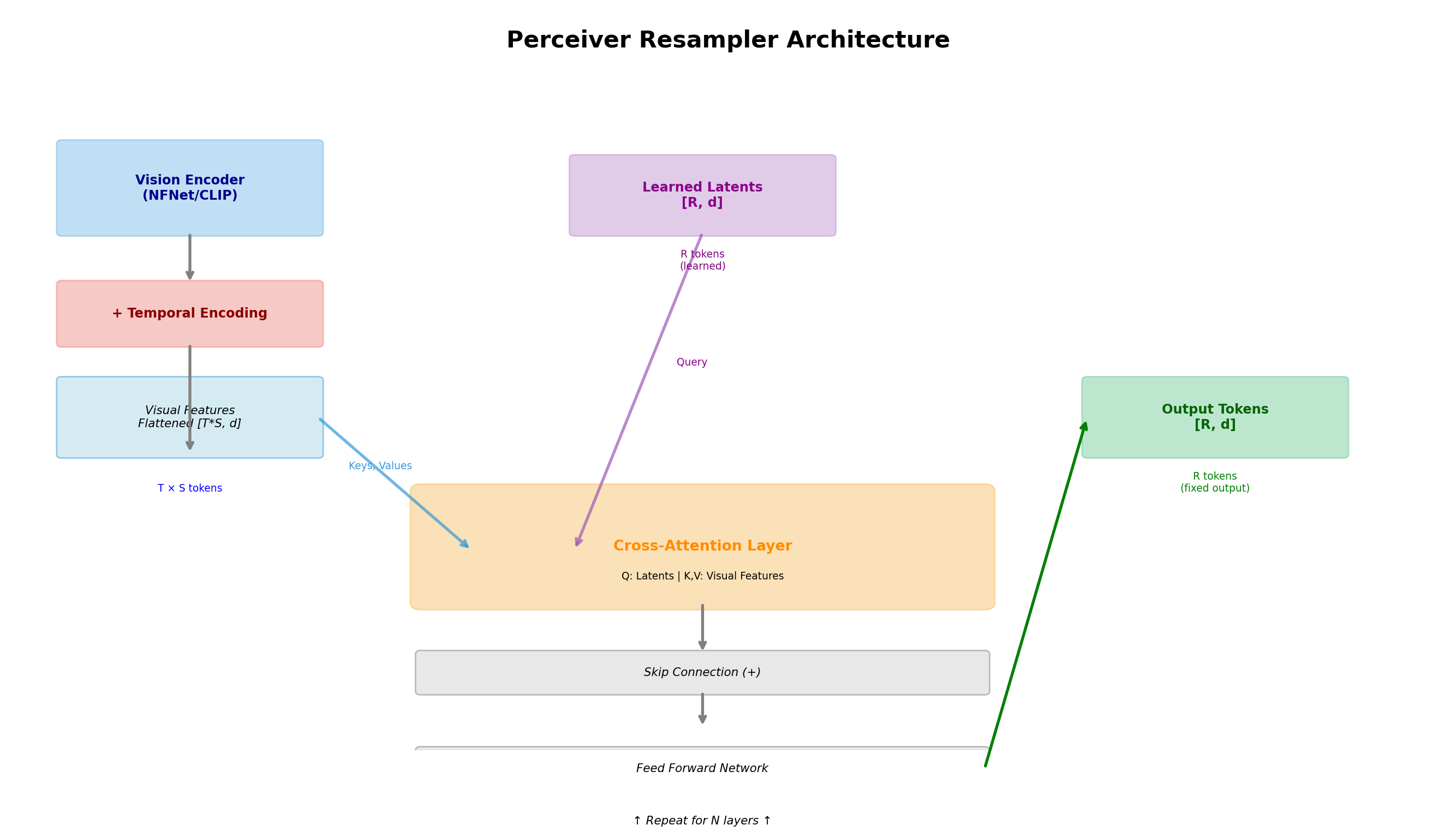
In the Perceiver Resampler: - Queries (Q): Our learned latents (fixed size, e.g., 64 tokens) - Keys (K) & Values (V): Visual features from the image encoder (variable size)

3.2 The Database Query Analogy

Think of cross-attention as querying a database:

Component Database Analogy Perceiver Resampler
Query Your search question Learned latent vectors (what to extract)
Key Database index Visual feature indices (what’s available)
Value Actual data Visual feature values (the information)
Attention Weights Relevance scores How much each feature contributes
import matplotlib.pyplot as plt
import matplotlib.patches as mpatches
from matplotlib.patches import FancyBboxPatch, FancyArrowPatch

def draw_cross_attention_flow():
    """Visualize cross-attention as a database query"""
    fig, ax = plt.subplots(figsize=(14, 6))
    ax.set_xlim(0, 14)
    ax.set_ylim(0, 6)
    ax.axis('off')

    # Title
    ax.text(7, 5.5, 'Cross-Attention: Database Query View', 
            ha='center', fontsize=16, weight='bold')

    # Visual Features (Database)
    db_box = FancyBboxPatch((0.5, 2), 3, 2.5, boxstyle="round,pad=0.1",
                            edgecolor='#3498db', facecolor='#3498db', alpha=0.3)
    ax.add_patch(db_box)
    ax.text(2, 4.5, 'Visual Features\n(Database)', ha='center', va='center',
            fontsize=11, weight='bold', color='darkblue')
    
    # Add feature tokens visualization
    for i in range(5):
        y_pos = 4.0 - i * 0.35
        rect = plt.Rectangle((0.7, y_pos), 2.6, 0.25, 
                            facecolor='lightblue', edgecolor='blue', alpha=0.6)
        ax.add_patch(rect)
        ax.text(2, y_pos + 0.125, f'Feature {i+1}', ha='center', va='center', fontsize=7)
    
    ax.text(2, 2.2, 'Keys & Values\n(Variable: M tokens)', ha='center', 
            fontsize=9, style='italic', color='darkblue')

    # Learned Latents (Queries)
    query_box = FancyBboxPatch((5.5, 2.5), 2.5, 2, boxstyle="round,pad=0.1",
                               edgecolor='#e74c3c', facecolor='#e74c3c', alpha=0.3)
    ax.add_patch(query_box)
    ax.text(6.75, 4.2, 'Learned Latents\n(Queries)', ha='center', va='center',
            fontsize=11, weight='bold', color='darkred')
    
    # Add latent tokens
    for i in range(3):
        y_pos = 3.7 - i * 0.4
        rect = plt.Rectangle((5.7, y_pos), 2.1, 0.3, 
                            facecolor='lightcoral', edgecolor='red', alpha=0.6)
        ax.add_patch(rect)
        ax.text(6.75, y_pos + 0.15, f'Latent {i+1}', ha='center', va='center', fontsize=8)
    
    ax.text(6.75, 2.7, 'Fixed: N tokens\n(N << M)', ha='center', 
            fontsize=9, style='italic', color='darkred')

    # Cross-Attention Operation
    attn_box = FancyBboxPatch((9, 2.5), 2, 2, boxstyle="round,pad=0.1",
                              edgecolor='#f39c12', facecolor='#f39c12', alpha=0.3)
    ax.add_patch(attn_box)
    ax.text(10, 4.2, 'Cross-Attention\nOperation', ha='center', va='center',
            fontsize=10, weight='bold', color='darkorange')
    ax.text(10, 3.5, 'softmax(QK^T/√d)V', ha='center', fontsize=9)
    ax.text(10, 3.0, 'O(M×N) complexity', ha='center', fontsize=8, style='italic')
    ax.text(10, 2.7, '(vs O(M²))', ha='center', fontsize=8, style='italic', color='green')

    # Output
    output_box = FancyBboxPatch((11.5, 2.5), 2, 2, boxstyle="round,pad=0.1",
                                edgecolor='#27ae60', facecolor='#27ae60', alpha=0.3)
    ax.add_patch(output_box)
    ax.text(12.5, 4.2, 'Output\nRepresentation', ha='center', va='center',
            fontsize=11, weight='bold', color='darkgreen')
    
    for i in range(3):
        y_pos = 3.7 - i * 0.4
        rect = plt.Rectangle((11.7, y_pos), 1.6, 0.3, 
                            facecolor='lightgreen', edgecolor='green', alpha=0.6)
        ax.add_patch(rect)
        ax.text(12.5, y_pos + 0.15, f'Output {i+1}', ha='center', va='center', fontsize=8)
    
    ax.text(12.5, 2.7, 'Fixed: N tokens', ha='center', 
            fontsize=9, style='italic', color='darkgreen')

    # Arrows
    ax.annotate('', xy=(5.5, 3.5), xytext=(3.5, 3.5),
                arrowprops=dict(arrowstyle='->', lw=2.5, color='purple'))
    ax.text(4.5, 3.8, 'K, V', ha='center', fontsize=10, color='purple', weight='bold')

    ax.annotate('', xy=(9, 3.5), xytext=(8, 3.5),
                arrowprops=dict(arrowstyle='->', lw=2.5, color='red'))
    ax.text(8.5, 3.8, 'Q', ha='center', fontsize=10, color='red', weight='bold')

    ax.annotate('', xy=(11.5, 3.5), xytext=(11, 3.5),
                arrowprops=dict(arrowstyle='->', lw=2.5, color='green'))

    plt.tight_layout()
    plt.show()

draw_cross_attention_flow()

The process:

  1. Query asks: “What information do I need?” (learned latents)
  2. Key responds: “Here’s what I have available” (visual features index)
  3. Value delivers: “Here’s the actual information” (visual feature values)
  4. Attention weights determine: “How much each value contributes” (learned relevance)

Part 4: Architecture Deep Dive

4.1 The Complete Perceiver Resampler

Let’s break down the full architecture, component by component:

def draw_perceiver_architecture():
    """Draw a detailed architecture diagram of the Perceiver Resampler"""
    fig, ax = plt.subplots(figsize=(16, 10))
    ax.set_xlim(0, 16)
    ax.set_ylim(0, 10)
    ax.axis('off')

    # Colors
    vision_color = '#3498db'
    time_color = '#e74c3c'
    latent_color = '#9b59b6'
    attn_color = '#f39c12'
    output_color = '#27ae60'
    fourier_color = '#e67e22'

    # Title
    ax.text(8, 9.5, 'Perceiver Resampler: Complete Architecture', 
            ha='center', fontsize=18, weight='bold')

    # Input
    input_box = FancyBboxPatch((0.5, 7.5), 3, 1, boxstyle="round,pad=0.05",
                               edgecolor='gray', facecolor='lightgray', alpha=0.5)
    ax.add_patch(input_box)
    ax.text(2, 8, 'Input: T frames × S patches × d dims', 
            ha='center', va='center', fontsize=10, weight='bold')

    # Step 1: Vision Encoder
    vision_box = FancyBboxPatch((0.5, 6), 3, 1, boxstyle="round,pad=0.05",
                                edgecolor=vision_color, facecolor=vision_color, alpha=0.3)
    ax.add_patch(vision_box)
    ax.text(2, 6.5, 'Vision Encoder\n(NFNet / CLIP / ViT)', 
            ha='center', va='center', fontsize=10, weight='bold', color='darkblue')

    # Arrow
    ax.annotate('', xy=(2, 6), xytext=(2, 7.5), 
                arrowprops=dict(arrowstyle='->', lw=2, color='gray'))

    # Step 2: Fourier Features (NEW!)
    fourier_box = FancyBboxPatch((0.5, 4.8), 3, 0.7, boxstyle="round,pad=0.05",
                                 edgecolor=fourier_color, facecolor=fourier_color, alpha=0.3)
    ax.add_patch(fourier_box)
    ax.text(2, 5.15, '+ Fourier Position Features', 
            ha='center', va='center', fontsize=9, weight='bold', color='darkorange')

    ax.annotate('', xy=(2, 5.5), xytext=(2, 6), 
                arrowprops=dict(arrowstyle='->', lw=2, color='gray'))

    # Step 3: Temporal Encoding
    time_box = FancyBboxPatch((0.5, 4), 3, 0.5, boxstyle="round,pad=0.05",
                              edgecolor=time_color, facecolor=time_color, alpha=0.3)
    ax.add_patch(time_box)
    ax.text(2, 4.25, '+ Learned Temporal Encoding', 
            ha='center', va='center', fontsize=9, weight='bold', color='darkred')

    ax.annotate('', xy=(2, 4.5), xytext=(2, 4.8), 
                arrowprops=dict(arrowstyle='->', lw=2, color='gray'))

    # Visual Features (flattened)
    features_box = FancyBboxPatch((0.5, 2.8), 3, 0.8, boxstyle="round,pad=0.05",
                                  edgecolor=vision_color, facecolor='lightblue', alpha=0.5)
    ax.add_patch(features_box)
    ax.text(2, 3.2, 'Visual Features\nFlattened [T×S, d]', 
            ha='center', va='center', fontsize=9, style='italic')
    ax.text(2, 2.9, 'M = T×S tokens (variable)', ha='center', fontsize=8, color='blue')

    ax.annotate('', xy=(2, 3.6), xytext=(2, 4), 
                arrowprops=dict(arrowstyle='->', lw=2, color='gray'))

    # Learned Latents (parallel path)
    latent_box = FancyBboxPatch((6.5, 6.5), 3, 1.2, boxstyle="round,pad=0.05",
                                edgecolor=latent_color, facecolor=latent_color, alpha=0.3)
    ax.add_patch(latent_box)
    ax.text(8, 7.3, 'Learned Latents', ha='center', va='center',
            fontsize=11, weight='bold', color='darkmagenta')
    ax.text(8, 6.95, '[N, d] - Fixed size', ha='center', va='center', fontsize=9)
    ax.text(8, 6.7, 'N << M (e.g., 64 << 2000)', ha='center', va='center', 
            fontsize=8, style='italic', color='purple')

    # Initialize note
    ax.text(8, 6.2, 'Initialized randomly,\nlearned via gradients', 
            ha='center', va='center', fontsize=8, style='italic', color='gray')

    # Cross-Attention Block
    attn_box = FancyBboxPatch((5, 2.5), 6, 1.8, boxstyle="round,pad=0.1",
                              edgecolor=attn_color, facecolor=attn_color, alpha=0.3)
    ax.add_patch(attn_box)
    ax.text(8, 3.8, 'Cross-Attention Layer', ha='center', va='center',
            fontsize=12, weight='bold', color='darkorange')
    ax.text(8, 3.4, 'Q: Latents [N, d] | K,V: Features [M, d]', ha='center', va='center', fontsize=9)
    ax.text(8, 3.0, 'Output: [N, d] - Fixed size!', ha='center', va='center', 
            fontsize=9, weight='bold', color='green')

    # Arrows to attention
    ax.annotate('', xy=(5.5, 3.4), xytext=(3.5, 3.4),
                arrowprops=dict(arrowstyle='->', lw=2.5, color=vision_color, alpha=0.8))
    ax.text(4.5, 3.7, 'K, V', fontsize=9, color=vision_color, weight='bold')

    ax.annotate('', xy=(7.5, 3.6), xytext=(7.5, 6.5),
                arrowprops=dict(arrowstyle='->', lw=2.5, color=latent_color, alpha=0.8))
    ax.text(7.2, 5.2, 'Q', fontsize=9, color='darkmagenta', weight='bold')

    # Self-Attention in Latent Space
    self_attn_box = FancyBboxPatch((5, 0.8), 6, 1.2, boxstyle="round,pad=0.05",
                                   edgecolor='gray', facecolor='lightgray', alpha=0.5)
    ax.add_patch(self_attn_box)
    ax.text(8, 1.6, 'Self-Attention in Latent Space', ha='center', va='center',
            fontsize=11, weight='bold')
    ax.text(8, 1.25, 'Deep processing: O(L×N²)', ha='center', va='center', fontsize=9)
    ax.text(8, 0.95, 'L layers, independent of input size!', ha='center', va='center', 
            fontsize=8, style='italic', color='green')

    ax.annotate('', xy=(8, 2.0), xytext=(8, 2.5),
                arrowprops=dict(arrowstyle='->', lw=2, color='gray'))

    # Feed Forward
    ff_box = FancyBboxPatch((5, -0.3), 6, 0.6, boxstyle="round,pad=0.05",
                           edgecolor='gray', facecolor='lightgray', alpha=0.5)
    ax.add_patch(ff_box)
    ax.text(8, 0, 'Feed Forward + LayerNorm + Residual', ha='center', va='center', fontsize=9)

    ax.annotate('', xy=(8, 0.2), xytext=(8, 0.8),
                arrowprops=dict(arrowstyle='->', lw=2, color='gray'))

    # Iteration indicator
    ax.text(8, -0.8, '↑ Repeat for L layers (e.g., 4-8) ↑', 
            ha='center', fontsize=10, style='italic', weight='bold')

    # Output
    output_box = FancyBboxPatch((12, 2.5), 3.5, 1.5, boxstyle="round,pad=0.05",
                                edgecolor=output_color, facecolor=output_color, alpha=0.3)
    ax.add_patch(output_box)
    ax.text(13.75, 3.5, 'Final Output', ha='center', va='center',
            fontsize=12, weight='bold', color='darkgreen')
    ax.text(13.75, 3.1, '[N, d] - Fixed size', ha='center', va='center', fontsize=10)
    ax.text(13.75, 2.8, 'Ready for Language Model!', ha='center', va='center', 
            fontsize=9, style='italic', color='green')

    # Arrow from FF loop to output
    ax.annotate('', xy=(12, 3.25), xytext=(11, 0),
                arrowprops=dict(arrowstyle='->', lw=2.5, color='green'))

    # Complexity annotations
    ax.text(2, 0.5, 'Input side:\nO(M×d)', ha='center', fontsize=8, 
            color='blue', style='italic')
    ax.text(8, -1.5, 'Latent side:\nO(L×N²×d)', ha='center', fontsize=8, 
            color='purple', style='italic')
    ax.text(13.75, 1.5, 'Total:\nO(M×N + L×N²)', ha='center', fontsize=9, 
            color='green', weight='bold')

    plt.tight_layout()
    plt.show()

draw_perceiver_architecture()

4.2 Step-by-Step Breakdown

Step 1: Vision Encoding

# Vision encoder output shape
# T = number of temporal frames (images)
# S = spatial tokens per image (e.g., 17×17 = 289 for ViT)
# d = feature dimension (e.g., 1024)
T, S, d = 8, 289, 1024  # Example: 8 frames, 289 patches per frame

visual_features = torch.randn(T, S, d)
print(f"Visual features shape: {visual_features.shape}")
print(f"Total tokens: {T * S:,}")
# Output: torch.Size([8, 289, 1024]) - 8 images, 289 tokens each = 2,312 tokens
Visual features shape: torch.Size([8, 289, 1024])
Total tokens: 2,312

Step 2: Fourier Position Features ⭐ NEW

The Perceiver uses Fourier features to encode spatial positions. This is crucial because attention is permutation-invariant—it doesn’t know where pixels are located!

def fourier_features(positions, num_bands=64, max_resolution=224):
    """
    Generate Fourier feature position encodings.
    
    Args:
        positions: [..., D] position coordinates in [-1, 1]
        num_bands: Number of frequency bands
        max_resolution: Maximum resolution (Nyquist frequency)
    
    Returns:
        Fourier features [..., D * (2*num_bands + 1)]
    """
    # Frequency bands equally spaced from 1 to max_resolution/2
    freqs = torch.linspace(1, max_resolution / 2, num_bands)
    
    # Compute sin and cos for each frequency
    features = []
    for freq in freqs:
        features.append(torch.sin(freq * positions))
        features.append(torch.cos(freq * positions))
    
    # Concatenate with original positions
    features.append(positions)
    
    return torch.cat(features, dim=-1)

# Example for a 2D image
x_coords = torch.linspace(-1, 1, 17)  # 17 patches wide
y_coords = torch.linspace(-1, 1, 17)  # 17 patches tall
xx, yy = torch.meshgrid(x_coords, y_coords, indexing='ij')
positions = torch.stack([xx, yy], dim=-1)  # [17, 17, 2]

fourier_pos = fourier_features(positions, num_bands=64)
print(f"Position shape: {positions.shape}")
print(f"Fourier features shape: {fourier_pos.shape}")
print(f"Feature expansion: 2D position → {fourier_pos.shape[-1]}D features")
Position shape: torch.Size([17, 17, 2])
Fourier features shape: torch.Size([17, 17, 258])
Feature expansion: 2D position → 258D features
Why Fourier Features?

The paper explains: “We use a parameterization of Fourier features that allows us to (i) directly represent the position structure of the input data, (ii) control the number of frequency bands independently of the cutoff frequency, and (iii) uniformly sample all frequencies up to a target resolution.”

Key insight: Unlike learned position embeddings, Fourier features provide a deterministic, high-fidelity representation of position that generalizes better and doesn’t require learning.

Step 3: Flattening Space and Time

The Perceiver Resampler flattens the spatial and temporal dimensions into a single sequence:

# Add temporal encoding
encoded = visual_features  # After temporal encoding

# Flatten: [T, S, d] -> [T*S, d]
T, S, d = encoded.shape
visual_features_flat = encoded.reshape(T * S, d)
print(f"After flattening: {visual_features_flat.shape}")
print(f"M = T×S = {T * S} tokens (variable input size)")
After flattening: torch.Size([2312, 1024])
M = T×S = 2312 tokens (variable input size)

Why does this work?

  • Spatial information is encoded in the feature vectors themselves (via Fourier features)
  • Temporal information is explicitly added via learned temporal embeddings
  • The flattening is consistent, so the model learns to handle this specific ordering

Step 4: Temporal Position Encodings

class TemporalEncoding(nn.Module):
    """Learned temporal position encodings for video frames"""

    def __init__(self, max_frames: int = 8, feature_dim: int = 1024):
        super().__init__()
        # Learnable embedding for each time position
        self.temporal_embeds = nn.Parameter(torch.randn(max_frames, feature_dim))

    def forward(self, features: torch.Tensor) -> torch.Tensor:
        """
        Args:
            features: [T, S, d] tensor of visual features
        Returns:
            features with temporal encoding added: [T, S, d]
        """
        T = features.shape[0]
        
        # Add temporal encoding to each frame
        # For each frame t, add self.temporal_embeds[t] to all S spatial tokens
        encoded = features + self.temporal_embeds[:T].unsqueeze(1)
        
        return encoded

# Example usage
temporal_encoder = TemporalEncoding(max_frames=8, feature_dim=1024)
encoded_features = temporal_encoder(visual_features)
print(f"Encoded features shape: {encoded_features.shape}")
Encoded features shape: torch.Size([8, 289, 1024])
Interpolation at Inference Time

Here’s something fascinating: Flamingo was trained with 8 frames, but at inference, it processes 30 frames!

How? By interpolating the temporal embeddings:

# Trained with 8 frames, need 30
trained_embeds = temporal_encoder.temporal_embeds  # Shape: [8, 1024]

# Linear interpolate to get 30 embeddings
from torch.nn.functional import interpolate
inference_embeds = interpolate(
    trained_embeds.T.unsqueeze(0),  # [1, 1024, 8]
    size=30,
    mode='linear',
    align_corners=False
).squeeze(0).T  # [1024, 30]

This remarkable property allows the model to generalize to different frame counts!

Step 5: Cross-Attention Layer

class CrossAttentionLayer(nn.Module):
    """Cross-attention where latents query visual features"""

    def __init__(self, latent_dim: int = 1024, num_heads: int = 8):
        super().__init__()
        self.latent_dim = latent_dim
        self.num_heads = num_heads
        self.head_dim = latent_dim // num_heads

        # Query projection: from latents
        self.q_proj = nn.Linear(latent_dim, latent_dim)

        # Key and Value projections: from visual features
        self.k_proj = nn.Linear(latent_dim, latent_dim)
        self.v_proj = nn.Linear(latent_dim, latent_dim)

        # Output projection
        self.out_proj = nn.Linear(latent_dim, latent_dim)

    def forward(self, latents: torch.Tensor, visual_features: torch.Tensor) -> torch.Tensor:
        """
        Args:
            latents: [N, d] - learned latent queries
            visual_features: [M, d] - flattened visual features
        Returns:
            Updated latents: [N, d]
        """
        N = latents.shape[0]
        M = visual_features.shape[0]

        # Project to Q, K, V
        Q = self.q_proj(latents)      # [N, d]
        K = self.k_proj(visual_features)  # [M, d]
        V = self.v_proj(visual_features)  # [M, d]

        # Reshape for multi-head attention
        Q = Q.view(N, self.num_heads, self.head_dim).transpose(0, 1)  # [heads, N, head_dim]
        K = K.view(M, self.num_heads, self.head_dim).transpose(0, 1)  # [heads, M, head_dim]
        V = V.view(M, self.num_heads, self.head_dim).transpose(0, 1)  # [heads, M, head_dim]

        # Compute attention scores: Q @ K^T
        scores = torch.matmul(Q, K.transpose(-2, -1)) / (self.head_dim ** 0.5)  # [heads, N, M]

        # Apply softmax to get attention weights
        attn_weights = torch.softmax(scores, dim=-1)  # [heads, N, M]

        # Apply attention to values
        attended = torch.matmul(attn_weights, V)  # [heads, N, head_dim]

        # Merge heads
        attended = attended.transpose(0, 1).contiguous().view(N, self.latent_dim)  # [N, d]

        # Output projection
        output = self.out_proj(attended)

        return output

# Complexity check
N, M, d = 64, 2312, 1024  # Example dimensions
print(f"Cross-attention complexity: O(N×M) = O({N}×{M}) = O({N*M:,})")
print(f"Self-attention complexity: O(M²) = O({M}²) = O({M**2:,})")
print(f"Speedup: {M**2 / (N*M):.1f}x faster!")
Cross-attention complexity: O(N×M) = O(64×2312) = O(147,968)
Self-attention complexity: O(M²) = O(2312²) = O(5,345,344)
Speedup: 36.1x faster!

Step 6: The Complete Perceiver Resampler

class PerceiverResampler(nn.Module):
    """
    The Perceiver Resampler: compresses variable-length visual input
    into a fixed-size representation using learned latent queries.
    """

    def __init__(
        self,
        feature_dim: int = 1024,
        num_latents: int = 64,
        num_layers: int = 4,
        num_heads: int = 8,
        max_frames: int = 8,
        use_fourier: bool = True,
        num_fourier_bands: int = 64
    ):
        super().__init__()
        self.use_fourier = use_fourier

        # Learnable latent queries (THE KEY INNOVATION!)
        self.latents = nn.Parameter(torch.randn(num_latents, feature_dim))

        # Temporal encoding
        self.temporal_encoding = TemporalEncoding(max_frames, feature_dim)

        # Cross-attention layers
        self.cross_attn_layers = nn.ModuleList([
            CrossAttentionLayer(feature_dim, num_heads)
            for _ in range(num_layers)
        ])

        # Self-attention layers (in latent space)
        self.self_attn_layers = nn.ModuleList([
            nn.MultiheadAttention(feature_dim, num_heads, batch_first=True)
            for _ in range(num_layers)
        ])

        # Feed-forward networks
        self.ffns = nn.ModuleList([
            nn.Sequential(
                nn.Linear(feature_dim, feature_dim * 4),
                nn.GELU(),
                nn.Linear(feature_dim * 4, feature_dim)
            )
            for _ in range(num_layers)
        ])

        # Layer normalization
        self.layer_norms = nn.ModuleList([
            nn.LayerNorm(feature_dim)
            for _ in range(num_layers * 3)
        ])

    def forward(self, visual_features: torch.Tensor) -> torch.Tensor:
        """
        Args:
            visual_features: [T, S, d] - visual features from encoder
        Returns:
            resampled: [N, d] - fixed-size representation
        """
        # Add temporal encoding
        encoded = self.temporal_encoding(visual_features)  # [T, S, d]

        # Flatten spatial and temporal dimensions
        T, S, d = encoded.shape
        visual_flat = encoded.reshape(T * S, d)  # [T*S, d]

        # Initialize latents (learned parameter, not computed from input!)
        x = self.latents  # [N, d]

        # Process through layers
        for i, (cross_attn, self_attn, ffn) in enumerate(
            zip(self.cross_attn_layers, self.self_attn_layers, self.ffns)
        ):
            # Cross-attention with visual features
            cross_out = cross_attn(x, visual_flat)
            x = x + self.layer_norms[3*i](cross_out)

            # Self-attention in latent space
            self_out, _ = self_attn(x.unsqueeze(0), x.unsqueeze(0), x.unsqueeze(0))
            x = x + self.layer_norms[3*i+1](self_out.squeeze(0))

            # Feed-forward
            ff_out = ffn(x)
            x = x + self.layer_norms[3*i+2](ff_out)

        return x  # [N, d] - same size as latents!

# Example usage
print("=" * 60)
print("PERCEIVER RESAMPLER DEMO")
print("=" * 60)

resampler = PerceiverResampler(
    feature_dim=1024,
    num_latents=64,
    num_layers=4,
    num_heads=8
)

# Process 8 frames
visual_input = torch.randn(8, 289, 1024)  # T=8, S=289, d=1024
output = resampler(visual_input)

print(f"\nInput:  {visual_input.shape[0]} frames × {visual_input.shape[1]} tokens = {visual_input.shape[0] * visual_input.shape[1]} tokens")
print(f"Output: {output.shape[0]} tokens (fixed size!)")
print(f"Compression ratio: {(visual_input.shape[0] * visual_input.shape[1]) / output.shape[0]:.1f}:1")
============================================================
PERCEIVER RESAMPLER DEMO
============================================================

Input:  8 frames × 289 tokens = 2312 tokens
Output: 64 tokens (fixed size!)
Compression ratio: 36.1:1

Part 5: Complexity Analysis

5.1 The Big-O Breakdown

Understanding why the Perceiver Resampler is efficient:

Operation Complexity Description
Standard Self-Attention \(O(M^2 d)\) All tokens attend to all tokens
Perceiver Cross-Attention \(O(M N d)\) Latents attend to all tokens
Latent Self-Attention \(O(L N^2 d)\) Deep processing in latent space
Total Perceiver \(O(M N + L N^2) d\) Linear in input, quadratic in latents

Where: - \(M\) = input tokens (variable, e.g., 2,000) - \(N\) = latent tokens (fixed, e.g., 64) - \(L\) = number of layers (e.g., 4-8) - \(d\) = feature dimension

def compare_complexity():
    """Visualize complexity comparison"""
    fig, (ax1, ax2) = plt.subplots(1, 2, figsize=(14, 5))

    # Complexity vs input size
    M_values = np.array([100, 500, 1000, 2000, 5000, 10000])
    N = 64  # Fixed latent size
    L = 6   # Number of layers

    self_attn = M_values ** 2
    perceiver = M_values * N + L * N ** 2

    ax1.plot(M_values, self_attn / 1e6, 'b-', linewidth=2.5, label='Self-Attention: O(M²)')
    ax1.plot(M_values, perceiver / 1e6, 'r-', linewidth=2.5, label='Perceiver: O(MN + LN²)')
    ax1.set_xlabel('Input Size (M tokens)', fontsize=12)
    ax1.set_ylabel('Complexity (millions of ops)', fontsize=12)
    ax1.set_title('Complexity vs Input Size', fontsize=13, weight='bold')
    ax1.legend(fontsize=11)
    ax1.grid(True, alpha=0.3)
    ax1.set_yscale('log')

    # Speedup ratio
    speedup = self_attn / perceiver
    ax2.bar(range(len(M_values)), speedup, color='green', alpha=0.7, edgecolor='darkgreen')
    ax2.set_xticks(range(len(M_values)))
    ax2.set_xticklabels([f'{m}' for m in M_values])
    ax2.set_xlabel('Input Size (M tokens)', fontsize=12)
    ax2.set_ylabel('Speedup Factor', fontsize=12)
    ax2.set_title('Perceiver Speedup vs Self-Attention', fontsize=13, weight='bold')
    ax2.grid(True, alpha=0.3, axis='y')

    # Add value labels on bars
    for i, v in enumerate(speedup):
        ax2.text(i, v + 0.5, f'{v:.1f}×', ha='center', va='bottom', fontsize=9, weight='bold')

    plt.tight_layout()
    plt.show()

    # Print specific example
    M = 2312  # 8 frames × 289 patches
    N = 64
    L = 6

    print("\n" + "=" * 60)
    print("COMPLEXITY COMPARISON (M=2312, N=64, L=6)")
    print("=" * 60)
    print(f"Self-Attention:  O(M²)     = O({M:,}²)     = O({M**2:>15,})")
    print(f"Perceiver:       O(MN+LN²) = O({M}×{N}+{L}×{N}²) = O({M*N + L*N**2:>15,})")
    print(f"Speedup:         {M**2 / (M*N + L*N**2):.1f}×")
    print("=" * 60)

compare_complexity()


============================================================
COMPLEXITY COMPARISON (M=2312, N=64, L=6)
============================================================
Self-Attention:  O(M²)     = O(2,312²)     = O(      5,345,344)
Perceiver:       O(MN+LN²) = O(2312×64+6×64²) = O(        172,544)
Speedup:         31.0×
============================================================

Part 6: The “Soft Clustering” Intuition

6.1 Understanding What Latents Learn

You might wonder: What do these learned latents actually represent?

The Perceiver paper describes this beautifully: the latents act like cluster centers in a soft clustering algorithm. Each latent specializes in extracting a certain type of information.

def visualize_latent_specialization():
    """Conceptual visualization of how latents might specialize"""
    fig, axes = plt.subplots(2, 4, figsize=(14, 7))
    fig.suptitle('How Learned Latents Might Specialize\n(Conceptual)', 
                 fontsize=14, weight='bold')

    # Conceptual specializations
    specializations = [
        ("Object Detector", "focuses on discrete objects"),
        ("Action Analyzer", "captures motion and activity"),
        ("Spatial Mapper", "understands spatial relationships"),
        ("Color Specialist", "attends to color patterns"),
        ("Texture Expert", "focuses on surface properties"),
        ("Scene Context", "understands overall context"),
        ("Temporal Tracker", "tracks changes over time"),
        ("Global Integrator", "holistic scene understanding")
    ]

    np.random.seed(42)
    for idx, (ax, (name, desc)) in enumerate(zip(axes.flat, specializations)):
        # Create a conceptual attention pattern
        attn_pattern = np.random.rand(16, 16)
        # Make it look more like real attention (some structure)
        center = (7, 7)
        for i in range(16):
            for j in range(16):
                dist = np.sqrt((i-center[0])**2 + (j-center[1])**2)
                attn_pattern[i, j] *= np.exp(-dist / 5)

        attn_pattern = attn_pattern / attn_pattern.sum()

        im = ax.imshow(attn_pattern, cmap='viridis', aspect='auto')
        ax.set_title(f'Latent {idx+1}: {name}\n{desc}', fontsize=9)
        ax.axis('off')

    plt.tight_layout()
    plt.show()

    print("\n" + "=" * 70)
    print("LATENT SPECIALIZATION EXAMPLES")
    print("=" * 70)
    examples = [
        "Latent 1: Attends to object boundaries and shapes",
        "Latent 2: Focuses on human figures and poses",
        "Latent 3: Tracks moving objects across frames",
        "Latent 4: Identifies background scene context",
        "...",
        "Latent 64: Captures fine-grained texture details"
    ]
    for ex in examples:
        print(f"  • {ex}")
    print("=" * 70)

visualize_latent_specialization()


======================================================================
LATENT SPECIALIZATION EXAMPLES
======================================================================
  • Latent 1: Attends to object boundaries and shapes
  • Latent 2: Focuses on human figures and poses
  • Latent 3: Tracks moving objects across frames
  • Latent 4: Identifies background scene context
  • ...
  • Latent 64: Captures fine-grained texture details
======================================================================

Key insight from the paper:

“The latent vectors in this case act as queries which extract information from the input data and need to be aligned in such a way that they extract the necessary information to perform the prediction task.”

Through training, gradients flow back and adjust these latents so they ask “better questions”—questions that extract information useful for the task at hand.

Not Traditional Clustering!

The Perceiver authors call this “end-to-end clustering” but it’s important to understand:

  • NOT K-means or any traditional clustering algorithm
  • NOT pre-computed from features
  • IS a soft, differentiable clustering that emerges from gradient descent
  • IS task-dependent—latents learn to cluster information relevant to the task

The “clusters” are implicit in the attention patterns that develop during training!


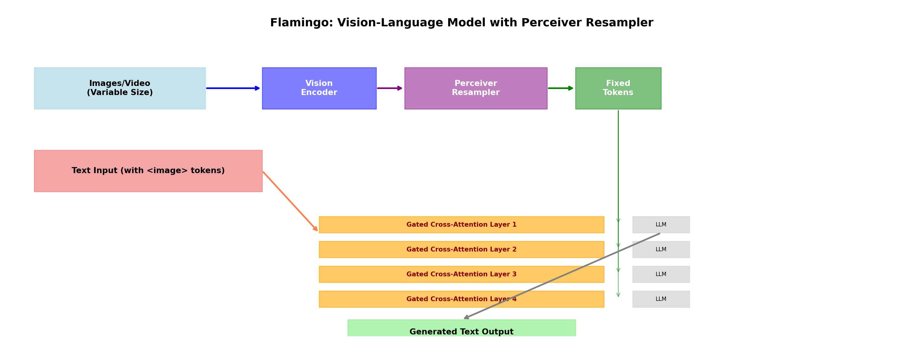
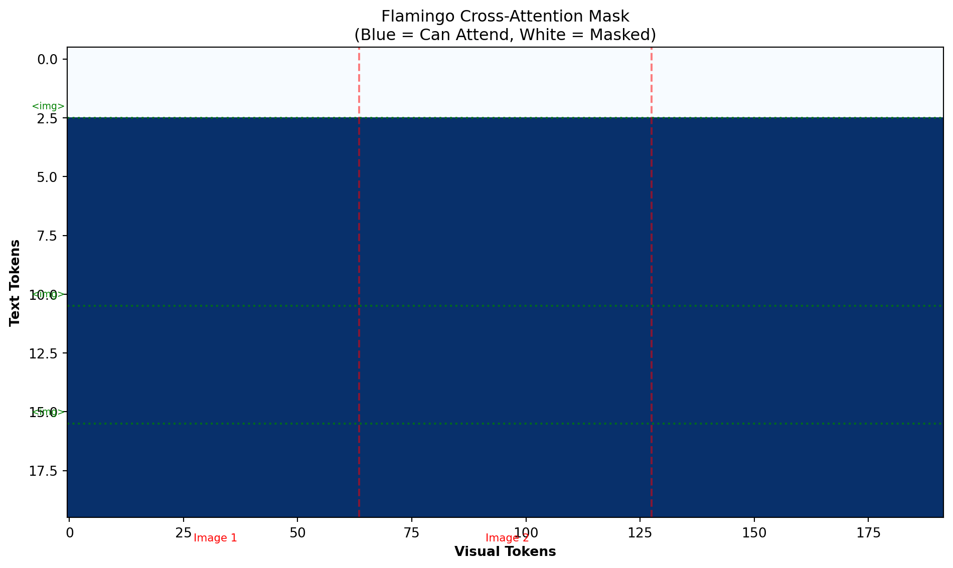
Part 7: The Flamingo Integration

7.1 How Flamingo Uses the Perceiver Resampler

The Perceiver Resampler was popularized by DeepMind’s Flamingo model. Let’s see how it fits into the complete architecture:

def draw_flamingo_architecture():
    """Draw the Flamingo architecture showing Perceiver Resampler integration"""
    fig, ax = plt.subplots(figsize=(16, 8))
    ax.set_xlim(0, 16)
    ax.set_ylim(0, 8)
    ax.axis('off')

    # Title
    ax.text(8, 7.5, 'Flamingo: Vision-Language Model with Perceiver Resampler',
            ha='center', fontsize=15, weight='bold')

    # Input Images
    ax.add_patch(plt.Rectangle((0.5, 6), 3, 1, fill=True, 
                               color='lightblue', alpha=0.7, edgecolor='blue', linewidth=2))
    ax.text(2, 6.5, 'Images/Video\n(Variable Size)', 
            ha='center', va='center', weight='bold', fontsize=10)

    # Vision Encoder
    ax.add_patch(plt.Rectangle((4, 6), 2.5, 1, fill=True, 
                               color='blue', alpha=0.6, edgecolor='darkblue', linewidth=2))
    ax.text(5.25, 6.5, 'Vision\nEncoder', 
            ha='center', va='center', weight='bold', color='white', fontsize=10)

    # Perceiver Resampler
    ax.add_patch(plt.Rectangle((7, 6), 3, 1, fill=True, 
                               color='purple', alpha=0.6, edgecolor='darkmagenta', linewidth=2))
    ax.text(8.5, 6.5, 'Perceiver\nResampler', 
            ha='center', va='center', weight='bold', color='white', fontsize=10)

    # Fixed visual tokens
    ax.add_patch(plt.Rectangle((10.5, 6), 2.5, 1, fill=True, 
                               color='green', alpha=0.6, edgecolor='darkgreen', linewidth=2))
    ax.text(11.75, 6.5, 'Fixed Visual\nTokens (64)', 
            ha='center', va='center', weight='bold', color='white', fontsize=10)

    # Arrows for vision path
    ax.annotate('', xy=(4, 6.5), xytext=(3.5, 6.5), 
                arrowprops=dict(arrowstyle='->', lw=2.5, color='blue'))
    ax.annotate('', xy=(7, 6.5), xytext=(6.5, 6.5), 
                arrowprops=dict(arrowstyle='->', lw=2.5, color='purple'))
    ax.annotate('', xy=(10.5, 6.5), xytext=(10, 6.5), 
                arrowprops=dict(arrowstyle='->', lw=2.5, color='green'))

    # Text input
    ax.add_patch(plt.Rectangle((0.5, 4), 4, 1, fill=True, 
                               color='lightcoral', alpha=0.7, edgecolor='red', linewidth=2))
    ax.text(2.5, 4.5, 'Text Input\n(with <image> tokens)', 
            ha='center', va='center', weight='bold', fontsize=10)

    # Gated Cross-Attention layers
    for i in range(4):
        y_pos = 3.2 - i * 0.6
        # Gated Cross-Attention
        ax.add_patch(plt.Rectangle((5.5, y_pos), 5, 0.45, fill=True, 
                                   color='orange', alpha=0.7, edgecolor='darkorange', linewidth=1.5))
        ax.text(8, y_pos + 0.225, f'Gated Cross-Attention {i+1}', 
                ha='center', va='center', fontsize=9, weight='bold', color='darkred')

        # LLM block
        ax.add_patch(plt.Rectangle((11, y_pos), 1.2, 0.45, fill=True, 
                                   color='lightgray', alpha=0.8, edgecolor='gray', linewidth=1.5))
        ax.text(11.6, y_pos + 0.225, 'LLM', 
                ha='center', va='center', fontsize=8, weight='bold')

    # Output
    ax.add_patch(plt.Rectangle((6, 0.5), 4, 0.8, fill=True, 
                               color='lightgreen', alpha=0.7, edgecolor='green', linewidth=2))
    ax.text(8, 0.9, 'Generated Text Output', 
            ha='center', va='center', weight='bold', fontsize=11)

    # Arrows
    # Vision to cross-attention
    for i in range(4):
        y_pos = 3.42 - i * 0.6
        ax.annotate('', xy=(11.5, y_pos), xytext=(11.5, 6), 
                    arrowprops=dict(arrowstyle='->', lw=1.5, color='green', alpha=0.6))

    # Text to first layer
    ax.annotate('', xy=(5.5, 3.2), xytext=(4.5, 4), 
                arrowprops=dict(arrowstyle='->', lw=2, color='coral'))

    # Layer connections
    for i in range(3):
        y_start = 3.2 - i * 0.6
        y_end = 2.6 - i * 0.6
        ax.annotate('', xy=(8, y_end), xytext=(8, y_start), 
                    arrowprops=dict(arrowstyle='->', lw=1.5, color='gray'))

    # To output
    ax.annotate('', xy=(8, 1.3), xytext=(11.6, 1.4), 
                arrowprops=dict(arrowstyle='->', lw=2, color='darkgreen'))

    # Labels
    ax.text(8, 5.5, '↓ Visual tokens attend to all text positions ↓', 
            ha='center', fontsize=9, style='italic', color='green')

    plt.tight_layout()
    plt.show()

draw_flamingo_architecture()

7.2 Gated Cross-Attention: Mixing Vision and Language

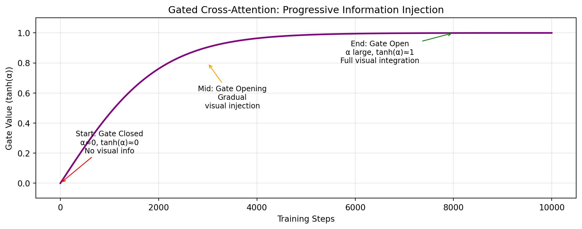
After the Perceiver Resampler produces fixed-size visual tokens, Flamingo uses gated cross-attention to inject this information into the language model:

class GatedCrossAttention(nn.Module):
    """
    Cross-attention with gating for controlled visual information injection.
    The gate starts closed (alpha=0) and gradually opens during training.
    """

    def __init__(self, lang_dim: int = 4096, visual_dim: int = 1024, num_heads: int = 8):
        super().__init__()
        self.cross_attn = nn.MultiheadAttention(
            embed_dim=lang_dim,
            num_heads=num_heads,
            batch_first=True
        )

        # Learnable gate parameter (initialized to 0 = closed)
        self.alpha = nn.Parameter(torch.zeros(1))

    def forward(self, lang_tokens: torch.Tensor, visual_tokens: torch.Tensor) -> torch.Tensor:
        """
        Args:
            lang_tokens: [batch, seq_len, lang_dim] - language model tokens
            visual_tokens: [batch, num_visual, visual_dim] - resampled visual tokens
        Returns:
            Updated lang_tokens with visual information injected
        """
        # Cross-attention: language queries, visual keys/values
        attn_out, _ = self.cross_attn(
            query=lang_tokens,
            key=visual_tokens,
            value=visual_tokens
        )

        # Tanh gate: controls how much visual information flows through
        # tanh(0) = 0 (closed), tanh(large) ≈ 1 (open)
        gate = torch.tanh(self.alpha)
        gated_output = gate * attn_out

        # Skip connection: preserve original language understanding
        return lang_tokens + gated_output

# Simulate training progression
print("\n" + "=" * 60)
print("GATED CROSS-ATTENTION: TRAINING PROGRESSION")
print("=" * 60)

# Training steps
steps = [0, 1000, 3000, 5000, 8000, 10000]
alpha_values = [0, 0.5, 1.5, 2.5, 4.0, 5.0]

print(f"{'Step':<10} {'α (raw)':<10} {'tanh(α) (gate)':<15} {'Visual Info Flow'}")
print("-" * 60)
for step, alpha in zip(steps, alpha_values):
    gate = np.tanh(alpha)
    bar = "█" * int(gate * 20)
    print(f"{step:<10} {alpha:<10.2f} {gate:<15.3f} {bar}")

print("=" * 60)

============================================================
GATED CROSS-ATTENTION: TRAINING PROGRESSION
============================================================
Step       α (raw)    tanh(α) (gate)  Visual Info Flow
------------------------------------------------------------
0          0.00       0.000           
1000       0.50       0.462           █████████
3000       1.50       0.905           ██████████████████
5000       2.50       0.987           ███████████████████
8000       4.00       0.999           ███████████████████
10000      5.00       1.000           ███████████████████
============================================================
Why the Gradual Gate?

When training Flamingo, the cross-attention gate starts closed (α=0 → tanh(α)=0). This is crucial:

  1. Protects the pre-trained LLM: The language model already knows how to process text—don’t disrupt it initially
  2. Allows gradual adaptation: Visual information is slowly integrated, preventing shock to the system
  3. Prevents catastrophic forgetting: The LLM doesn’t suddenly “forget” how to handle text
  4. Stabilizes training: The model learns to balance textual and visual information gradually

It’s like introducing a new team member gradually rather than throwing them into the deep end!


Part 8: Training Tips & Common Pitfalls

8.1 Best Practices

✅ DO: Recommended Practices

Latent Initialization: - Use small random initialization (std ~0.02) - Truncated normal with bounds [-2, 2] works well - The paper found performance is robust to initialization scale

Architecture Choices: - num_latents: 32-128 (64 is a good default) - num_layers: 4-6 for most applications - num_heads: 8 is standard - feature_dim: Match your vision encoder output (usually 768 or 1024)

Training Tips: - Use learning rate warmup for latents (they’re learning “from scratch”) - Consider layer-wise learning rate decay - Weight sharing across layers reduces overfitting significantly

❌ DON’T: Common Pitfalls

Initialization Issues: - Don’t initialize latents with large values (can cause instability) - Don’t use zero initialization (no gradient flow initially)

Architecture Mistakes: - Don’t make N (num_latents) too small (<32) - bottleneck too aggressive - Don’t make N too large (>512) - loses the efficiency benefit - Don’t forget temporal encodings for video - model won’t understand time!

Training Mistakes: - Don’t freeze latents initially - they need to learn! - Don’t use too high learning rate for latents - they’re sensitive - Don’t forget to interpolate temporal embeddings when using different frame counts

8.2 Hyperparameter Guide

import pandas as pd

# Create a hyperparameter reference table
hyperparams = {
    'Hyperparameter': [
        'num_latents (N)',
        'num_layers (L)',
        'num_heads',
        'feature_dim (d)',
        'max_frames'
    ],
    'Typical Values': [
        '64 (Flamingo)',
        '4-6',
        '8',
        '1024',
        '8 (trainable)'
    ],
    'Effect': [
        'More latents → more info, but slower',
        'More layers → deeper processing',
        'More heads → richer attention patterns',
        'Larger → more expressive',
        'Higher → need interpolation at inference'
    ],
    'Sweet Spot': [
        '32-128 (task-dependent)',
        '4-6 (diminishing returns after)',
        '8 (standard)',
        '768-1024 (match encoder)',
        '8 (interpolate beyond)'
    ]
}

df = pd.DataFrame(hyperparams)
print("\nHYPERPARAMETER REFERENCE TABLE")
print("=" * 80)
print(df.to_string(index=False))
print("=" * 80)

HYPERPARAMETER REFERENCE TABLE
================================================================================
 Hyperparameter Typical Values                                   Effect                      Sweet Spot
num_latents (N)  64 (Flamingo)     More latents → more info, but slower         32-128 (task-dependent)
 num_layers (L)            4-6          More layers → deeper processing 4-6 (diminishing returns after)
      num_heads              8   More heads → richer attention patterns                    8 (standard)
feature_dim (d)           1024                 Larger → more expressive        768-1024 (match encoder)
     max_frames  8 (trainable) Higher → need interpolation at inference          8 (interpolate beyond)
================================================================================

Part 9: Summary & Quick Reference

9.1 Core Concepts

Concept Description Key Insight
Learned Latents Randomly initialized, task-specialized query vectors NOT computed from input—learned via gradients!
Cross-Attention Latents query visual features Q=latents, K,V=features; complexity O(MN)
Temporal Encoding Learned vectors added to each frame Enables video understanding; can interpolate!
Fourier Features Position encodings using sinusoids Provides high-fidelity spatial information
Information Bottleneck Variable input → Fixed output Forces model to learn task-relevant compression

9.2 Architecture Flow

┌─────────────────────────────────────────────────────────────┐
│                    PERCEIVER RESAMPLER                       │
├─────────────────────────────────────────────────────────────┤
│  Input: T frames × S patches × d dims                        │
│       ↓                                                      │
│  Vision Encoder (NFNet/ViT/CLIP)                             │
│       ↓                                                      │
│  + Fourier Position Features (spatial)                       │
│  + Temporal Encoding (learned, temporal)                     │
│       ↓                                                      │
│  Flatten: [T×S, d] = [M, d]  (M = variable input size)       │
│       ↓                                                      │
│  Cross-Attention: Q=[N,d], K,V=[M,d] → [N,d]                 │
│       ↓                                                      │
│  Self-Attention in Latent Space (L layers, O(LN²))           │
│       ↓                                                      │
│  Output: [N, d]  (N = fixed, N << M)                         │
│       ↓                                                      │
│  Ready for Language Model!                                   │
└─────────────────────────────────────────────────────────────┘

9.3 Key Equations

Cross-Attention: \[ \text{CrossAttn}(Q, K, V) = \text{softmax}\left(\frac{QK^T}{\sqrt{d_k}}\right)V \]

With learned latents as queries: \[ Q = \text{Latents} \in \mathbb{R}^{N \times d} \quad \text{(learned parameters)} \] \[ K, V = \text{VisualFeatures} \in \mathbb{R}^{M \times d} \quad \text{(from encoder)} \]

Complexity: \[ \text{Total} = O(M \cdot N \cdot d) + O(L \cdot N^2 \cdot d) \ll O(M^2 \cdot d) \]


Part 10: Further Reading & Resources

Congratulations! You Now Understand the Perceiver Resampler! 🎉

You’ve learned:

  • ✅ The problem of variable-length visual input and quadratic attention
  • ✅ How learned latent queries create an efficient information bottleneck
  • ✅ Cross-attention as a differentiable database query mechanism
  • ✅ Temporal encodings and Fourier features for position information
  • ✅ The Flamingo integration and gated cross-attention
  • ✅ Practical implementation details and training tips

Further Reading:

  1. Perceiver: General Perception with Iterative Attention - The original paper by Jaegle et al. (DeepMind, 2021)
  2. Flamingo: a Visual Language Model for Few-Shot Learning - Application to VLM by Alayrac et al. (DeepMind, 2022)
  3. Perceiver IO - Follow-up with output cross-attention
  4. Set Transformer - Precursor work on cross-attention for sets

Acknowledgments

This blog is based on insights from: - The Perceiver paper by Jaegle et al. (DeepMind, 2021) - The Flamingo paper by Alayrac et al. (DeepMind, 2022) - The Set Transformer paper by Lee et al. (2019) - The excellent explainer by Daniel Warfield on Flamingo - StackExchange discussions on learned latents


Happy Learning! May your attention mechanisms always attend to what matters! 🎯

Questions or feedback? Feel free to reach out or open an issue on GitHub!