Random Variables, PMF, CDF, and Expectation: From Intuition to Implementation

A complete guide to the building blocks of probability theory with NumPy examples and practice problems

Probability Theory Fundamentals

Random Variables, PMF, CDF, and Expectation

Part 1: Random Variables

1.1 Thinking Lens

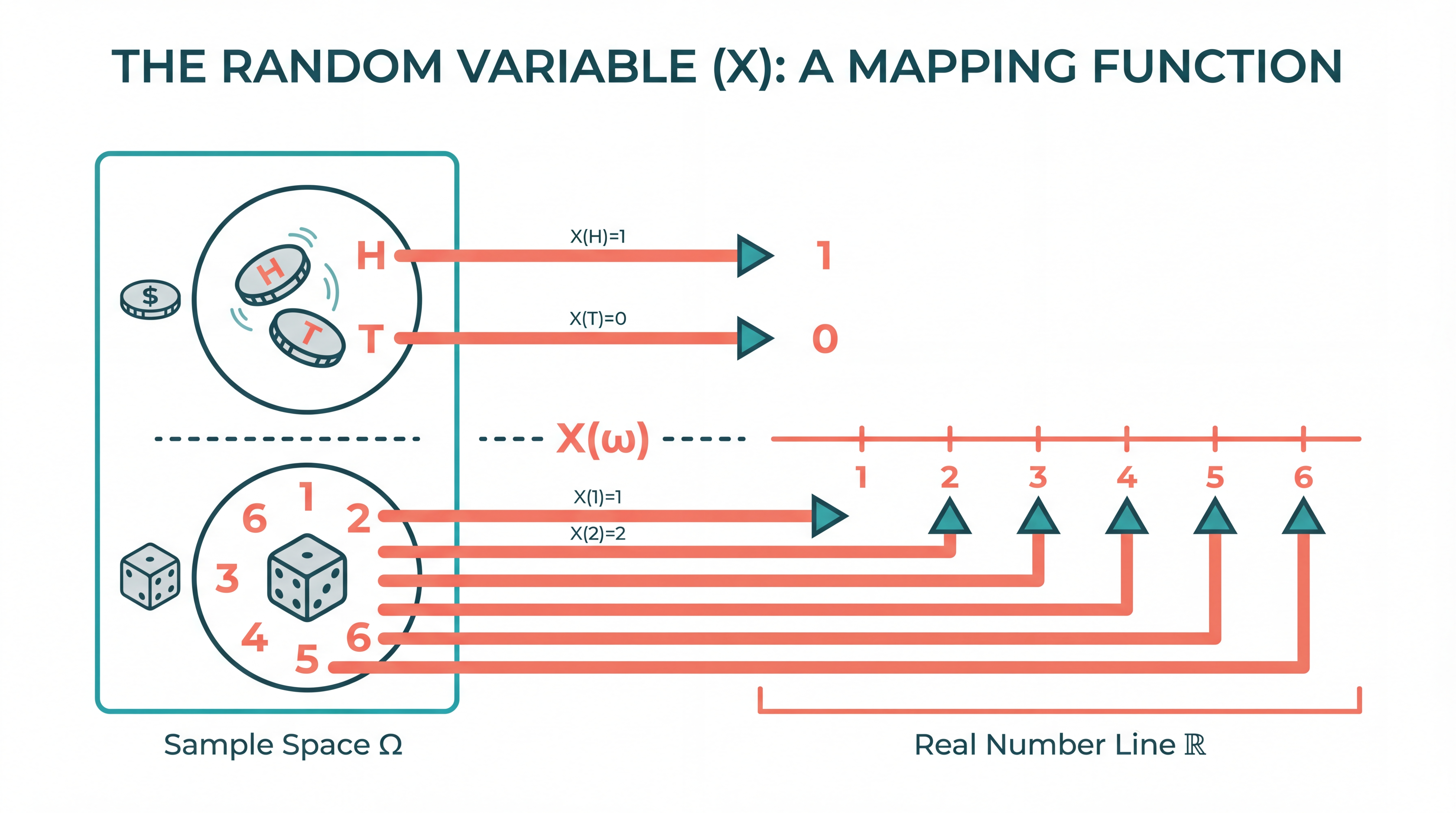
When you flip a coin, the outcome is “Heads” or “Tails”. When you roll a die, the outcome is a face with dots. These are words and images, not numbers. But mathematics works with numbers.

A random variable is a translator. It takes outcomes from the real world and converts them into numbers that we can compute with.

Think of it like a scoring system:

• Coin flip: Heads → 1, Tails → 0
• Die roll: Each face → its dot count (1, 2, 3, 4, 5, 6)
• Customer arrival: Each customer → time they arrived

The randomness comes from the underlying experiment (the coin flip, the die roll). The “variable” part is the numerical assignment.

A random variable is a function that assigns a real number to each outcome of a random experiment.

1.2 Definition

Formally, a random variable \(X\) is a function:

\[ X: \Omega \rightarrow \mathbb{R} \]

Where:

• \(\Omega\) is the sample space (set of all possible outcomes)
• \(\mathbb{R}\) is the set of real numbers

For each outcome \(\omega \in \Omega\), \(X(\omega)\) gives us a real number.

Types of Random Variables:

Type	Values	Example
Discrete	Countable (finite or infinite)	Die roll: {1, 2, 3, 4, 5, 6}
Continuous	Uncountable (any value in an interval)	Height: any value in [0, 300] cm

A random variable maps outcomes from the sample space to real numbers, enabling mathematical analysis of random phenomena.

1.3 Code: Random Variables in NumPy

import numpy as np
import matplotlib.pyplot as plt
from scipy import stats

np.random.seed(42)

# Example 1: Coin flip as a random variable
# Sample space: {Heads, Tails}
# Random variable X: Heads -> 1, Tails -> 0

def coin_flip_rv(n_flips=10):
    """Simulate coin flips as random variable values."""
    outcomes = np.random.choice(['Heads', 'Tails'], size=n_flips)
    # Map to numbers
    X = np.array([1 if o == 'Heads' else 0 for o in outcomes])
    return outcomes, X

outcomes, X = coin_flip_rv(10)
print("Coin Flip Random Variable:")
print(f"  Outcomes: {outcomes}")
print(f"  X values: {X}")
print(f"  Sum (count of heads): {X.sum()}")

Coin Flip Random Variable:
  Outcomes: ['Heads' 'Tails' 'Heads' 'Heads' 'Heads' 'Tails' 'Heads' 'Heads' 'Heads'
 'Tails']
  X values: [1 0 1 1 1 0 1 1 1 0]
  Sum (count of heads): 7

# Example 2: Die roll as a random variable
# The random variable IS the face value

def die_roll_rv(n_rolls=10):
    """Die roll - the outcome is already a number."""
    X = np.random.randint(1, 7, size=n_rolls)
    return X

X_die = die_roll_rv(10)
print("\nDie Roll Random Variable:")
print(f"  X values: {X_die}")
print(f"  Mean: {X_die.mean():.2f}")

Die Roll Random Variable:
  X values: [3 3 3 5 4 3 6 5 2 4]
  Mean: 3.80

# Example 3: Sum of two dice
# Random variable Y = X1 + X2

def two_dice_sum_rv(n_rolls=10):
    """Sum of two dice - a function of two random variables."""
    X1 = np.random.randint(1, 7, size=n_rolls)
    X2 = np.random.randint(1, 7, size=n_rolls)
    Y = X1 + X2
    return X1, X2, Y

X1, X2, Y = two_dice_sum_rv(10)
print("\nSum of Two Dice:")
print(f"  Die 1: {X1}")
print(f"  Die 2: {X2}")
print(f"  Sum Y: {Y}")
print(f"  Possible values of Y: {set(range(2, 13))}")

Sum of Two Dice:
  Die 1: [6 6 2 4 5 1 4 2 6 5]
  Die 2: [4 1 1 3 3 2 4 4 6 6]
  Sum Y: [10  7  3  7  8  3  8  6 12 11]
  Possible values of Y: {2, 3, 4, 5, 6, 7, 8, 9, 10, 11, 12}

Key Insight

A random variable is NOT random by itself. The randomness comes from the underlying experiment. The variable is just a systematic way to assign numbers to outcomes.

Think: “Random experiment” + “Numerical assignment rule” = “Random variable”

Part 2: Probability Mass Function (PMF)

2.1 Thinking Lens

Once we have a random variable, we want to know: how likely is each value?

For discrete random variables, the PMF answers this question. It tells us the probability of the random variable taking each specific value.

Think of PMF as a “probability bar chart”:

• Each possible value gets a bar
• The height of each bar is the probability
• All bar heights must sum to 1

For a fair die:

• P(X = 1) = 1/6
• P(X = 2) = 1/6
• … and so on

The PMF completely describes the behavior of a discrete random variable.

2.2 Definition

The Probability Mass Function (PMF) of a discrete random variable \(X\) is:

\[ p_X(x) = P(X = x) \]

Properties of PMF:

1. Non-negativity: \(p_X(x) \geq 0\) for all \(x\)
2. Normalization: \(\sum_x p_X(x) = 1\)

For a fair die with \(X \in \{1, 2, 3, 4, 5, 6\}\):

\[ p_X(x) = \frac{1}{6} \quad \text{for } x \in \{1, 2, 3, 4, 5, 6\} \]

The PMF shows the probability of each discrete value. For a fair die, each outcome has equal probability 1/6.

2.3 Code: Computing and Visualizing PMF

# PMF of a fair die
def compute_pmf(X):
    """Compute empirical PMF from samples."""
    values, counts = np.unique(X, return_counts=True)
    pmf = counts / len(X)
    return values, pmf

# Simulate many die rolls
X_die = np.random.randint(1, 7, size=10000)
values, pmf = compute_pmf(X_die)

print("Empirical PMF of Fair Die (10,000 rolls):")
print("-" * 35)
for v, p in zip(values, pmf):
    bar = "█" * int(p * 50)
    print(f"  P(X = {v}) = {p:.4f} {bar}")
print(f"\nSum of PMF: {pmf.sum():.4f} (should be 1.0)")

Empirical PMF of Fair Die (10,000 rolls):
-----------------------------------
  P(X = 1) = 0.1667 ████████
  P(X = 2) = 0.1694 ████████
  P(X = 3) = 0.1622 ████████
  P(X = 4) = 0.1671 ████████
  P(X = 5) = 0.1689 ████████
  P(X = 6) = 0.1657 ████████

Sum of PMF: 1.0000 (should be 1.0)

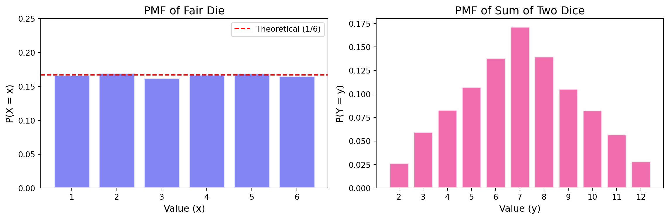
# Visualize PMF
fig, axes = plt.subplots(1, 2, figsize=(12, 4))

# Fair die PMF
ax = axes[0]
ax.bar(values, pmf, color='#6366f1', alpha=0.8, edgecolor='white', linewidth=2)
ax.axhline(y=1/6, color='red', linestyle='--', label='Theoretical (1/6)')
ax.set_xlabel('Value (x)', fontsize=12)
ax.set_ylabel('P(X = x)', fontsize=12)
ax.set_title('PMF of Fair Die', fontsize=14)
ax.set_xticks(range(1, 7))
ax.legend()
ax.set_ylim(0, 0.25)

# Sum of two dice PMF
X1 = np.random.randint(1, 7, size=10000)
X2 = np.random.randint(1, 7, size=10000)
Y = X1 + X2
values_y, pmf_y = compute_pmf(Y)

ax = axes[1]
ax.bar(values_y, pmf_y, color='#ec4899', alpha=0.8, edgecolor='white', linewidth=2)
ax.set_xlabel('Value (y)', fontsize=12)
ax.set_ylabel('P(Y = y)', fontsize=12)
ax.set_title('PMF of Sum of Two Dice', fontsize=14)
ax.set_xticks(range(2, 13))

plt.tight_layout()
plt.show()

# Theoretical PMF for sum of two dice
def theoretical_two_dice_pmf():
    """Compute exact PMF for sum of two fair dice."""
    pmf = {}
    for x1 in range(1, 7):
        for x2 in range(1, 7):
            s = x1 + x2
            pmf[s] = pmf.get(s, 0) + 1/36
    return pmf

theoretical = theoretical_two_dice_pmf()
print("Theoretical PMF for Sum of Two Dice:")
print("-" * 40)
for value in sorted(theoretical.keys()):
    prob = theoretical[value]
    bar = "█" * int(prob * 60)
    print(f"  P(Y = {value:2d}) = {prob:.4f} ({int(prob*36)}/36) {bar}")

Theoretical PMF for Sum of Two Dice:
----------------------------------------
  P(Y =  2) = 0.0278 (1/36) █
  P(Y =  3) = 0.0556 (2/36) ███
  P(Y =  4) = 0.0833 (3/36) █████
  P(Y =  5) = 0.1111 (4/36) ██████
  P(Y =  6) = 0.1389 (5/36) ████████
  P(Y =  7) = 0.1667 (6/36) ██████████
  P(Y =  8) = 0.1389 (5/36) ████████
  P(Y =  9) = 0.1111 (4/36) ██████
  P(Y = 10) = 0.0833 (3/36) █████
  P(Y = 11) = 0.0556 (2/36) ███
  P(Y = 12) = 0.0278 (1/36) █

Why 7 is most likely?

When rolling two dice, 7 has the most ways to occur: (1,6), (2,5), (3,4), (4,3), (5,2), (6,1) = 6 ways out of 36. That is why 7 appears most often in board games!

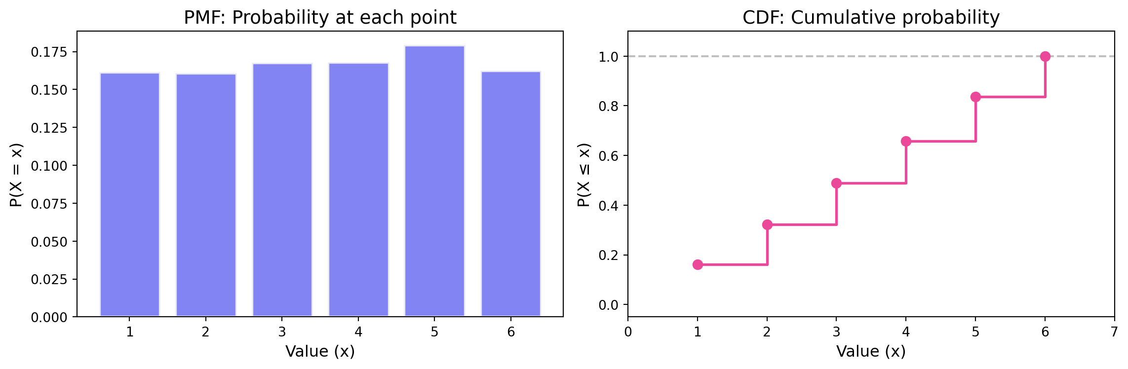
Part 3: Cumulative Distribution Function (CDF)

3.1 Thinking Lens

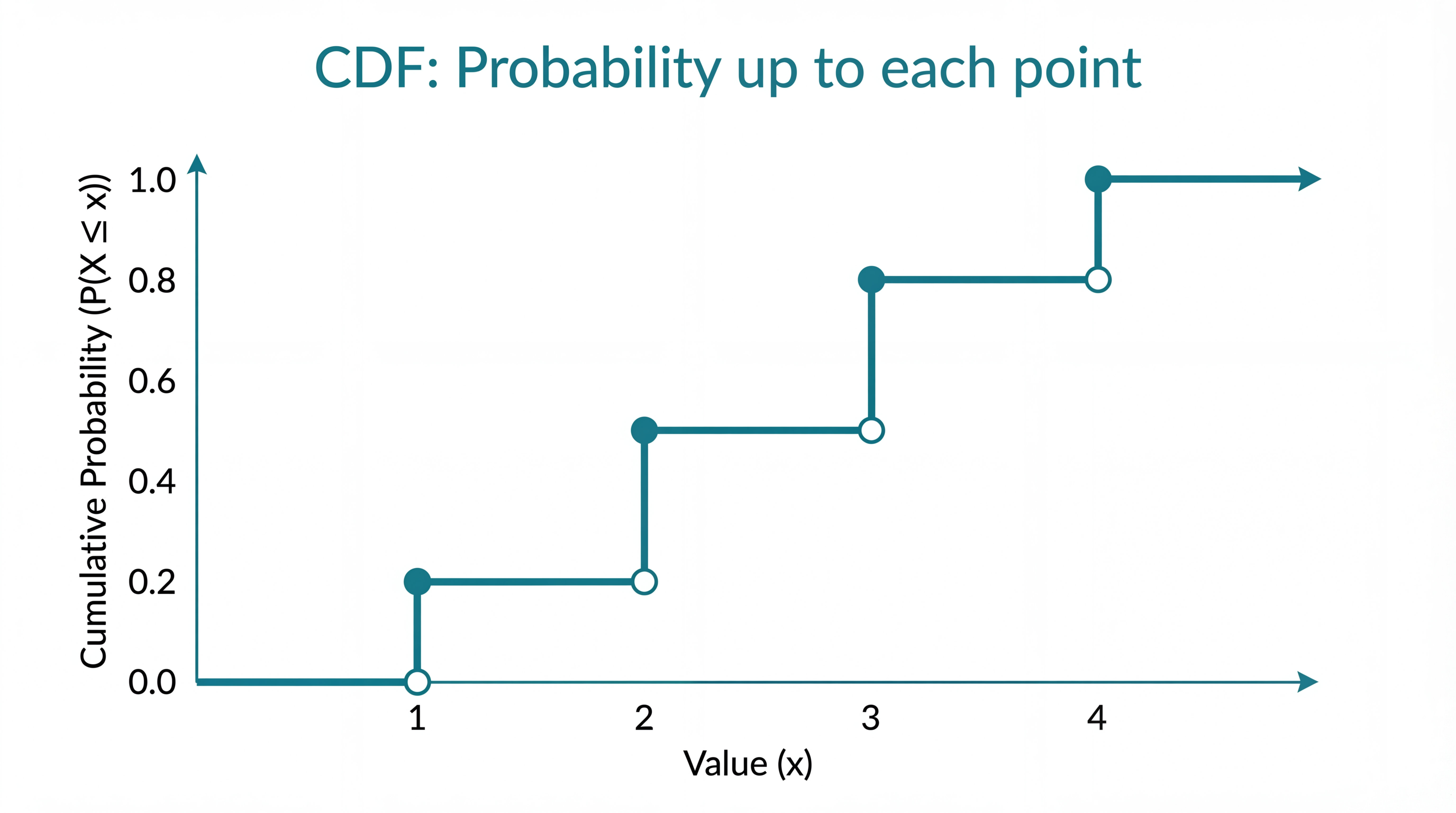
The PMF tells us the probability of exact values. But often we want to know: what is the probability of getting at most some value?

The CDF answers: “What is the probability that X is less than or equal to x?”

Think of it as accumulating probabilities:

• CDF at x = 1: P(X ≤ 1) = P(X = 1)
• CDF at x = 2: P(X ≤ 2) = P(X = 1) + P(X = 2)
• CDF at x = 3: P(X ≤ 3) = P(X = 1) + P(X = 2) + P(X = 3)
• … and so on

The CDF is a “running total” of probabilities.

Key property: CDF always goes from 0 to 1, never decreasing.

3.2 Definition

The Cumulative Distribution Function (CDF) of a random variable \(X\) is:

\[ F_X(x) = P(X \leq x) \]

Properties of CDF:

1. Non-decreasing: If \(a < b\), then \(F_X(a) \leq F_X(b)\)
2. Limits: \(\lim_{x \to -\infty} F_X(x) = 0\) and \(\lim_{x \to +\infty} F_X(x) = 1\)
3. Right-continuous: \(\lim_{h \to 0^+} F_X(x+h) = F_X(x)\)

Relationship to PMF (for discrete RVs):

\[ F_X(x) = \sum_{k \leq x} p_X(k) \]

Useful formulas:

\[ P(a < X \leq b) = F_X(b) - F_X(a) \]

\[ P(X > x) = 1 - F_X(x) \]

The CDF accumulates probabilities, showing P(X ≤ x) for each value x. It forms a step function for discrete random variables.

3.3 Code: Computing and Visualizing CDF

def compute_cdf(X):
    """Compute empirical CDF from samples."""
    sorted_X = np.sort(X)
    cdf = np.arange(1, len(X) + 1) / len(X)
    return sorted_X, cdf

def cdf_from_pmf(values, pmf):
    """Convert PMF to CDF."""
    cdf = np.cumsum(pmf)
    return values, cdf

# Fair die CDF
X_die = np.random.randint(1, 7, size=10000)
values, pmf = compute_pmf(X_die)
_, cdf = cdf_from_pmf(values, pmf)

print("CDF of Fair Die:")
print("-" * 40)
for v, c in zip(values, cdf):
    bar = "█" * int(c * 30)
    print(f"  P(X ≤ {v}) = {c:.4f} {bar}")

CDF of Fair Die:
----------------------------------------
  P(X ≤ 1) = 0.1615 ████
  P(X ≤ 2) = 0.3224 █████████
  P(X ≤ 3) = 0.4900 ██████████████
  P(X ≤ 4) = 0.6581 ███████████████████
  P(X ≤ 5) = 0.8375 █████████████████████████
  P(X ≤ 6) = 1.0000 ██████████████████████████████

# Visualize PMF and CDF side by side
fig, axes = plt.subplots(1, 2, figsize=(12, 4))

# PMF
ax = axes[0]
ax.bar(values, pmf, color='#6366f1', alpha=0.8, edgecolor='white', linewidth=2)
ax.set_xlabel('Value (x)', fontsize=12)
ax.set_ylabel('P(X = x)', fontsize=12)
ax.set_title('PMF: Probability at each point', fontsize=14)
ax.set_xticks(range(1, 7))

# CDF as step function
ax = axes[1]
# Create step function
x_steps = np.concatenate([[0], np.repeat(values, 2), [7]])
y_steps = np.concatenate([[0], np.repeat(cdf, 2)])
y_steps = np.insert(y_steps[:-1], 0, 0)

ax.step(values, cdf, where='post', color='#ec4899', linewidth=2, label='CDF')
ax.scatter(values, cdf, color='#ec4899', s=50, zorder=5)
ax.axhline(y=1, color='gray', linestyle='--', alpha=0.5)
ax.set_xlabel('Value (x)', fontsize=12)
ax.set_ylabel('P(X ≤ x)', fontsize=12)
ax.set_title('CDF: Cumulative probability', fontsize=14)
ax.set_xticks(range(0, 8))
ax.set_ylim(-0.05, 1.1)

plt.tight_layout()
plt.show()

# Using CDF for probability calculations
print("Using CDF to compute probabilities:")
print("-" * 45)

# P(X <= 3) for fair die
p_leq_3 = cdf[values == 3][0] if 3 in values else 0
print(f"P(X ≤ 3) = {p_leq_3:.4f} (theoretical: 0.5)")

# P(X > 4) = 1 - P(X <= 4)
p_gt_4 = 1 - cdf[values == 4][0] if 4 in values else 1
print(f"P(X > 4) = 1 - P(X ≤ 4) = {p_gt_4:.4f} (theoretical: 2/6 = 0.333)")

# P(2 < X <= 5) = P(X <= 5) - P(X <= 2)
p_2_to_5 = cdf[values == 5][0] - cdf[values == 2][0]
print(f"P(2 < X ≤ 5) = P(X ≤ 5) - P(X ≤ 2) = {p_2_to_5:.4f} (theoretical: 3/6 = 0.5)")

Using CDF to compute probabilities:
---------------------------------------------
P(X ≤ 3) = 0.4900 (theoretical: 0.5)
P(X > 4) = 1 - P(X ≤ 4) = 0.3419 (theoretical: 2/6 = 0.333)
P(2 < X ≤ 5) = P(X ≤ 5) - P(X ≤ 2) = 0.5151 (theoretical: 3/6 = 0.5)

CDF vs PMF: When to use which?

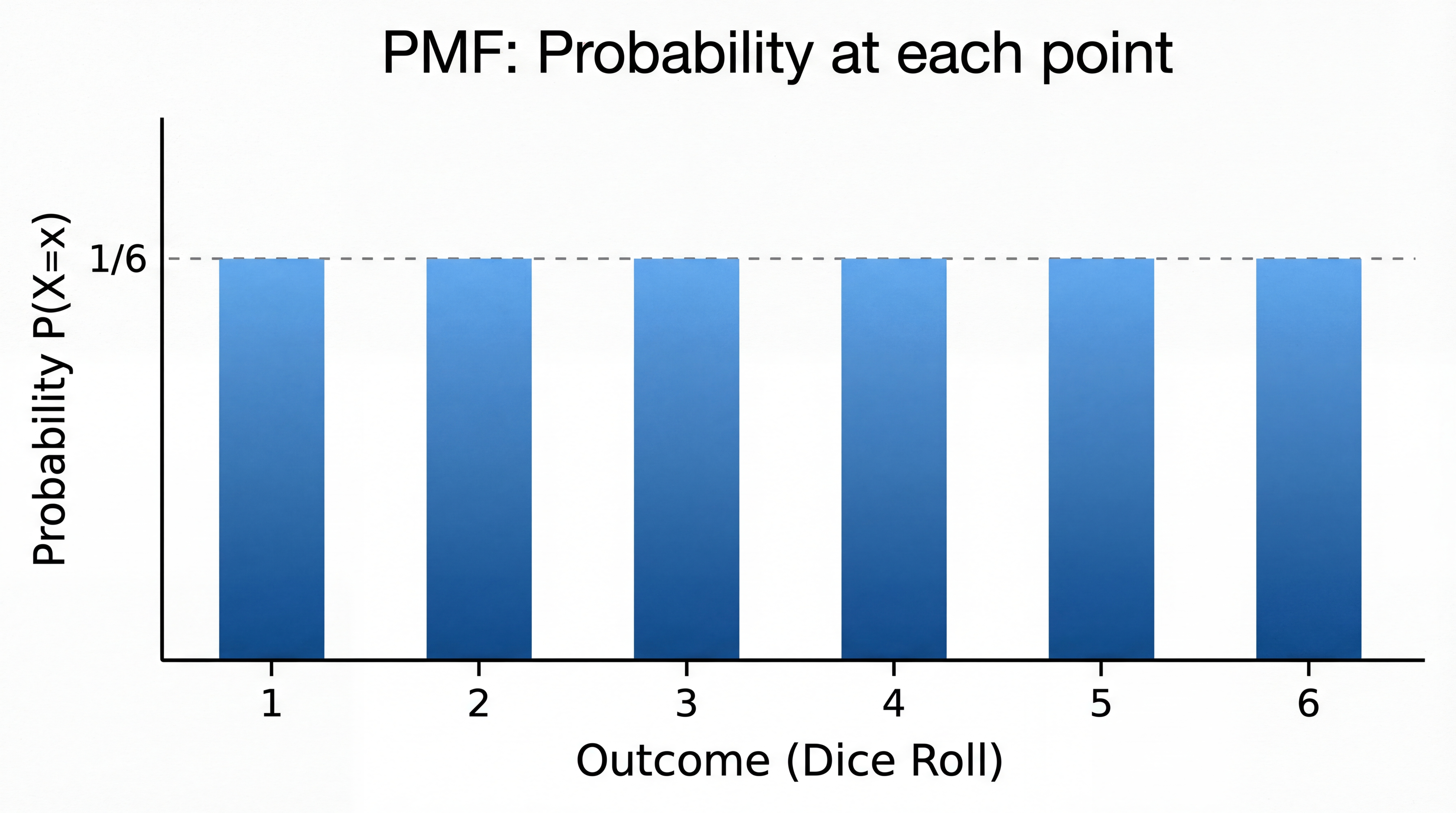
Use PMF when: - You want P(X = specific value) - You are working with discrete distributions - You want to visualize the probability distribution shape

Use CDF when: - You want P(X ≤ x) or P(X > x) or P(a < X ≤ b) - You are comparing distributions (CDFs are easier to compare) - You are generating random samples (inverse CDF method)

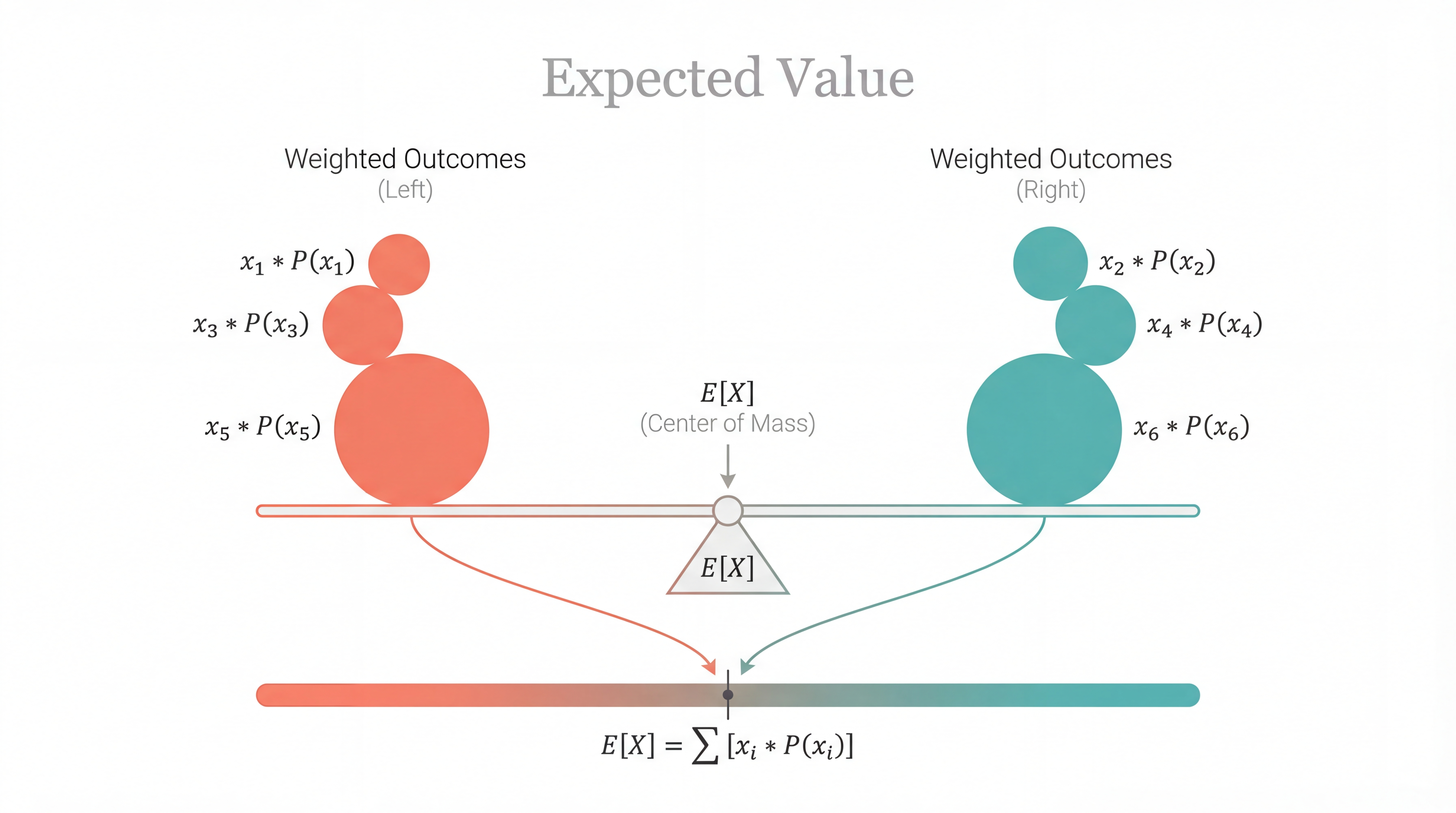
Part 4: Expectation (Expected Value)

4.1 Thinking Lens

If you rolled a fair die infinitely many times and averaged the results, what would you get?

The expectation (or expected value) is this theoretical “long-run average”. It is the center of mass of the probability distribution.

Think of it like this:

• Place weights on a number line
• Each value gets a weight equal to its probability
• The balance point (center of mass) is the expected value

For a fair die:

\[ E[X] = 1 \cdot \frac{1}{6} + 2 \cdot \frac{1}{6} + 3 \cdot \frac{1}{6} + 4 \cdot \frac{1}{6} + 5 \cdot \frac{1}{6} + 6 \cdot \frac{1}{6} = 3.5 \]

Notice: 3.5 is not even a possible outcome! The expected value is a weighted average, not necessarily a possible value.

4.2 Definition

The Expected Value (or Expectation or Mean) of a discrete random variable \(X\) is:

\[ E[X] = \mu_X = \sum_x x \cdot p_X(x) \]

Properties of Expectation:

1. Linearity: \(E[aX + b] = aE[X] + b\)
2. Additivity: \(E[X + Y] = E[X] + E[Y]\) (always true, even if X and Y are dependent)
3. For functions: \(E[g(X)] = \sum_x g(x) \cdot p_X(x)\)

Important derived quantities:

Variance: \(\text{Var}(X) = E[(X - \mu)^2] = E[X^2] - (E[X])^2\)

Standard Deviation: \(\sigma_X = \sqrt{\text{Var}(X)}\)

The expected value is the balance point (center of mass) of the probability distribution.

4.3 Code: Computing Expectations

def compute_expectation(values, pmf):
    """Compute expected value from PMF."""
    return np.sum(values * pmf)

def compute_variance(values, pmf):
    """Compute variance from PMF."""
    mu = compute_expectation(values, pmf)
    return np.sum((values - mu)**2 * pmf)

# Fair die
values_die = np.array([1, 2, 3, 4, 5, 6])
pmf_die = np.array([1/6, 1/6, 1/6, 1/6, 1/6, 1/6])

E_die = compute_expectation(values_die, pmf_die)
Var_die = compute_variance(values_die, pmf_die)

print("Fair Die Statistics:")
print("-" * 35)
print(f"  E[X] = {E_die:.4f}")
print(f"  Var(X) = {Var_die:.4f}")
print(f"  SD(X) = {np.sqrt(Var_die):.4f}")

Fair Die Statistics:
-----------------------------------
  E[X] = 3.5000
  Var(X) = 2.9167
  SD(X) = 1.7078

# Verify with simulation
X_samples = np.random.randint(1, 7, size=100000)

print("\nVerification with 100,000 samples:")
print(f"  Sample mean: {X_samples.mean():.4f}")
print(f"  Sample variance: {X_samples.var():.4f}")
print(f"  Sample std: {X_samples.std():.4f}")

Verification with 100,000 samples:
  Sample mean: 3.5037
  Sample variance: 2.9206
  Sample std: 1.7090

# Expected value of sum of two dice
# E[X + Y] = E[X] + E[Y] = 3.5 + 3.5 = 7

X1 = np.random.randint(1, 7, size=100000)
X2 = np.random.randint(1, 7, size=100000)
Y = X1 + X2

print("\nSum of Two Dice:")
print(f"  E[X1] = E[X2] = 3.5")
print(f"  E[X1 + X2] = E[X1] + E[X2] = 7.0")
print(f"  Sample mean of Y: {Y.mean():.4f}")

Sum of Two Dice:
  E[X1] = E[X2] = 3.5
  E[X1 + X2] = E[X1] + E[X2] = 7.0
  Sample mean of Y: 6.9896

# Expected value of a function of X
# E[X^2] for fair die

def compute_expectation_of_function(values, pmf, func):
    """Compute E[g(X)] for function g."""
    return np.sum(func(values) * pmf)

E_X_squared = compute_expectation_of_function(values_die, pmf_die, lambda x: x**2)

print("\nExpectation of X^2 (fair die):")
print(f"  E[X^2] = {E_X_squared:.4f}")
print(f"  Verify: Var(X) = E[X^2] - E[X]^2 = {E_X_squared} - {E_die**2} = {E_X_squared - E_die**2:.4f}")

Expectation of X^2 (fair die):
  E[X^2] = 15.1667
  Verify: Var(X) = E[X^2] - E[X]^2 = 15.166666666666666 - 12.25 = 2.9167

4.4 Code: Linearity of Expectation

# Demonstrate linearity: E[aX + b] = aE[X] + b
a, b = 2, 5

# Method 1: Transform and compute expectation
Y_samples = a * X_samples + b
E_Y_empirical = Y_samples.mean()

# Method 2: Use linearity formula
E_Y_theoretical = a * E_die + b

print("Linearity of Expectation: Y = 2X + 5")
print("-" * 40)
print(f"  E[X] = {E_die}")
print(f"  E[Y] = E[2X + 5] = 2*E[X] + 5 = 2*{E_die} + 5 = {E_Y_theoretical}")
print(f"  Empirical E[Y] = {E_Y_empirical:.4f}")

Linearity of Expectation: Y = 2X + 5
----------------------------------------
  E[X] = 3.5
  E[Y] = E[2X + 5] = 2*E[X] + 5 = 2*3.5 + 5 = 12.0
  Empirical E[Y] = 12.0074

Part 5: Common Discrete Distributions

5.1 Bernoulli Distribution

A single trial with two outcomes (success/failure).

\[ X \sim \text{Bernoulli}(p) \implies P(X = 1) = p, \quad P(X = 0) = 1-p \]

\[ E[X] = p, \quad \text{Var}(X) = p(1-p) \]

# Bernoulli distribution
p = 0.7
X_bernoulli = np.random.binomial(1, p, size=10000)

print("Bernoulli(p=0.7):")
print(f"  P(X=1) empirical: {(X_bernoulli == 1).mean():.4f}")
print(f"  P(X=0) empirical: {(X_bernoulli == 0).mean():.4f}")
print(f"  E[X] = {X_bernoulli.mean():.4f} (theoretical: {p})")
print(f"  Var(X) = {X_bernoulli.var():.4f} (theoretical: {p*(1-p)})")

Bernoulli(p=0.7):
  P(X=1) empirical: 0.6979
  P(X=0) empirical: 0.3021
  E[X] = 0.6979 (theoretical: 0.7)
  Var(X) = 0.2108 (theoretical: 0.21000000000000002)

5.2 Binomial Distribution

Number of successes in n independent Bernoulli trials.

\[ X \sim \text{Binomial}(n, p) \implies P(X = k) = \binom{n}{k} p^k (1-p)^{n-k} \]

\[ E[X] = np, \quad \text{Var}(X) = np(1-p) \]

# Binomial distribution
n, p = 10, 0.3
X_binomial = np.random.binomial(n, p, size=10000)

print(f"\nBinomial(n={n}, p={p}):")
print(f"  E[X] = {X_binomial.mean():.4f} (theoretical: {n*p})")
print(f"  Var(X) = {X_binomial.var():.4f} (theoretical: {n*p*(1-p)})")

# Plot PMF
fig, ax = plt.subplots(figsize=(10, 4))
values, pmf = compute_pmf(X_binomial)
ax.bar(values, pmf, color='#6366f1', alpha=0.8, edgecolor='white')

# Theoretical PMF
from scipy.stats import binom
x_theory = np.arange(0, n+1)
pmf_theory = binom.pmf(x_theory, n, p)
ax.plot(x_theory, pmf_theory, 'ro-', label='Theoretical', markersize=8)

ax.set_xlabel('Number of successes (k)')
ax.set_ylabel('P(X = k)')
ax.set_title(f'Binomial Distribution (n={n}, p={p})')
ax.legend()
plt.tight_layout()
plt.show()

Binomial(n=10, p=0.3):
  E[X] = 2.9925 (theoretical: 3.0)
  Var(X) = 2.1544 (theoretical: 2.0999999999999996)

5.3 Geometric Distribution

Number of trials until first success.

\[ X \sim \text{Geometric}(p) \implies P(X = k) = (1-p)^{k-1} p \]

\[ E[X] = \frac{1}{p}, \quad \text{Var}(X) = \frac{1-p}{p^2} \]

# Geometric distribution
p = 0.25
X_geometric = np.random.geometric(p, size=10000)

print(f"\nGeometric(p={p}):")
print(f"  E[X] = {X_geometric.mean():.4f} (theoretical: {1/p})")
print(f"  Var(X) = {X_geometric.var():.4f} (theoretical: {(1-p)/p**2})")

Geometric(p=0.25):
  E[X] = 3.9693 (theoretical: 4.0)
  Var(X) = 11.7870 (theoretical: 12.0)

5.4 Poisson Distribution

Number of events in a fixed interval (given average rate λ).

\[ X \sim \text{Poisson}(\lambda) \implies P(X = k) = \frac{\lambda^k e^{-\lambda}}{k!} \]

\[ E[X] = \lambda, \quad \text{Var}(X) = \lambda \]

# Poisson distribution
lam = 5
X_poisson = np.random.poisson(lam, size=10000)

print(f"\nPoisson(λ={lam}):")
print(f"  E[X] = {X_poisson.mean():.4f} (theoretical: {lam})")
print(f"  Var(X) = {X_poisson.var():.4f} (theoretical: {lam})")

# Note: For Poisson, E[X] = Var(X) = λ

Poisson(λ=5):
  E[X] = 5.0262 (theoretical: 5)
  Var(X) = 4.8993 (theoretical: 5)

Part 6: Practice Problems

Problem 1: Loaded Die

Problem

A loaded die has the following probabilities:

Face	1	2	3	4	5	6
P(X=x)	0.1	0.1	0.1	0.1	0.1	0.5

1. Verify this is a valid PMF.
2. Compute E[X].
3. Compute P(X ≥ 4).
4. Compute Var(X).

Solution

# Loaded die problem
values = np.array([1, 2, 3, 4, 5, 6])
pmf = np.array([0.1, 0.1, 0.1, 0.1, 0.1, 0.5])

# (a) Valid PMF check
print("(a) PMF validation:")
print(f"    All non-negative: {np.all(pmf >= 0)}")
print(f"    Sum = {pmf.sum():.1f} (should be 1)")

# (b) Expected value
E_X = compute_expectation(values, pmf)
print(f"\n(b) E[X] = {E_X:.2f}")

# (c) P(X >= 4)
P_geq_4 = pmf[values >= 4].sum()
print(f"\n(c) P(X ≥ 4) = P(X=4) + P(X=5) + P(X=6)")
print(f"    = 0.1 + 0.1 + 0.5 = {P_geq_4:.1f}")

# (d) Variance
Var_X = compute_variance(values, pmf)
print(f"\n(d) Var(X) = E[X²] - E[X]²")
E_X2 = compute_expectation_of_function(values, pmf, lambda x: x**2)
print(f"    E[X²] = {E_X2:.2f}")
print(f"    Var(X) = {E_X2:.2f} - {E_X:.2f}² = {Var_X:.2f}")

(a) PMF validation:
    All non-negative: True
    Sum = 1.0 (should be 1)

(b) E[X] = 4.50

(c) P(X ≥ 4) = P(X=4) + P(X=5) + P(X=6)
    = 0.1 + 0.1 + 0.5 = 0.7

(d) Var(X) = E[X²] - E[X]²
    E[X²] = 23.50
    Var(X) = 23.50 - 4.50² = 3.25

Problem 2: Maximum of Two Dice

Problem

Roll two fair dice. Let Y = max(X₁, X₂) be the maximum of the two values.

1. Find the PMF of Y.
2. Compute E[Y].
3. Compute P(Y ≤ 4).

Solution

# Maximum of two dice
# Y = max(X1, X2)

# Theoretical PMF
def pmf_max_two_dice():
    """P(Y = k) = P(max(X1,X2) = k)"""
    pmf = {}
    for k in range(1, 7):
        # P(Y = k) = P(Y <= k) - P(Y <= k-1)
        # P(Y <= k) = P(X1 <= k AND X2 <= k) = (k/6)^2
        p_leq_k = (k/6)**2
        p_leq_k_minus_1 = ((k-1)/6)**2 if k > 1 else 0
        pmf[k] = p_leq_k - p_leq_k_minus_1
    return pmf

pmf_Y = pmf_max_two_dice()

print("(a) PMF of Y = max(X1, X2):")
print("-" * 40)
for k, p in pmf_Y.items():
    print(f"    P(Y = {k}) = {p:.4f} = {int(p*36)}/36")

# (b) E[Y]
E_Y = sum(k * p for k, p in pmf_Y.items())
print(f"\n(b) E[Y] = {E_Y:.4f}")

# Verify with simulation
X1 = np.random.randint(1, 7, size=100000)
X2 = np.random.randint(1, 7, size=100000)
Y = np.maximum(X1, X2)
print(f"    Simulated E[Y] = {Y.mean():.4f}")

# (c) P(Y <= 4)
P_Y_leq_4 = sum(p for k, p in pmf_Y.items() if k <= 4)
print(f"\n(c) P(Y ≤ 4) = {P_Y_leq_4:.4f} = {int(P_Y_leq_4*36)}/36")
print(f"    Alternative: (4/6)² = {(4/6)**2:.4f}")

(a) PMF of Y = max(X1, X2):
----------------------------------------
    P(Y = 1) = 0.0278 = 1/36
    P(Y = 2) = 0.0833 = 3/36
    P(Y = 3) = 0.1389 = 5/36
    P(Y = 4) = 0.1944 = 6/36
    P(Y = 5) = 0.2500 = 9/36
    P(Y = 6) = 0.3056 = 10/36

(b) E[Y] = 4.4722
    Simulated E[Y] = 4.4708

(c) P(Y ≤ 4) = 0.4444 = 16/36
    Alternative: (4/6)² = 0.4444

Problem 3: Insurance Claims

Problem

An insurance company models the number of claims per day as a Poisson(λ=3) random variable. Each claim costs $1000.

1. What is the probability of exactly 5 claims in a day?
2. What is the expected daily cost?
3. What is the probability of more than 5 claims?

Solution

from scipy.stats import poisson

lam = 3
cost_per_claim = 1000

# (a) P(X = 5)
p_5 = poisson.pmf(5, lam)
print(f"(a) P(X = 5) = {p_5:.4f}")
print(f"    Formula: λ^5 * e^(-λ) / 5! = 3^5 * e^(-3) / 120")

# (b) Expected daily cost
# E[Cost] = E[1000 * X] = 1000 * E[X] = 1000 * λ
E_cost = cost_per_claim * lam
print(f"\n(b) E[Daily Cost] = 1000 × E[X] = 1000 × {lam} = ${E_cost}")

# (c) P(X > 5) = 1 - P(X <= 5)
p_gt_5 = 1 - poisson.cdf(5, lam)
print(f"\n(c) P(X > 5) = 1 - P(X ≤ 5) = {p_gt_5:.4f}")

# Verify with simulation
X_sim = np.random.poisson(lam, size=100000)
print(f"    Simulated: {(X_sim > 5).mean():.4f}")

(a) P(X = 5) = 0.1008
    Formula: λ^5 * e^(-λ) / 5! = 3^5 * e^(-3) / 120

(b) E[Daily Cost] = 1000 × E[X] = 1000 × 3 = $3000

(c) P(X > 5) = 1 - P(X ≤ 5) = 0.0839
    Simulated: 0.0848

Problem 4: Quality Control

Problem

A factory produces items with a 5% defect rate. A batch of 20 items is inspected.

1. What is the probability of exactly 2 defective items?
2. What is the probability of at most 2 defective items?
3. What is the expected number of defective items?
4. If each defective item costs $50 to fix, what is the expected repair cost per batch?

Solution

from scipy.stats import binom

n = 20  # batch size
p = 0.05  # defect rate
fix_cost = 50

# (a) P(X = 2)
p_2 = binom.pmf(2, n, p)
print(f"(a) P(X = 2) = {p_2:.4f}")

# (b) P(X <= 2)
p_leq_2 = binom.cdf(2, n, p)
print(f"\n(b) P(X ≤ 2) = P(X=0) + P(X=1) + P(X=2)")
print(f"    = {binom.pmf(0, n, p):.4f} + {binom.pmf(1, n, p):.4f} + {binom.pmf(2, n, p):.4f}")
print(f"    = {p_leq_2:.4f}")

# (c) E[X]
E_X = n * p
print(f"\n(c) E[X] = n × p = {n} × {p} = {E_X}")

# (d) Expected repair cost
E_cost = fix_cost * E_X
print(f"\n(d) E[Repair Cost] = $50 × E[X] = $50 × {E_X} = ${E_cost}")

(a) P(X = 2) = 0.1887

(b) P(X ≤ 2) = P(X=0) + P(X=1) + P(X=2)
    = 0.3585 + 0.3774 + 0.1887
    = 0.9245

(c) E[X] = n × p = 20 × 0.05 = 1.0

(d) E[Repair Cost] = $50 × E[X] = $50 × 1.0 = $50.0

Problem 5: Waiting for Success

Problem

A basketball player has a 40% free throw success rate. Let X be the number of attempts until the first successful shot.

1. What distribution does X follow?
2. What is P(X = 3)?
3. What is the expected number of attempts?
4. What is P(X > 5)?

Solution

from scipy.stats import geom

p = 0.4

print("(a) X follows Geometric(p=0.4)")
print("    X = number of trials until first success")

# (b) P(X = 3)
# P(X = 3) = (1-p)^2 * p = fail, fail, success
p_3 = geom.pmf(3, p)
print(f"\n(b) P(X = 3) = (1-p)² × p = 0.6² × 0.4 = {p_3:.4f}")

# (c) E[X]
E_X = 1 / p
print(f"\n(c) E[X] = 1/p = 1/{p} = {E_X:.2f}")

# (d) P(X > 5)
# P(X > 5) = probability of 5 consecutive failures = (1-p)^5
p_gt_5 = (1-p)**5
print(f"\n(d) P(X > 5) = P(first 5 are failures)")
print(f"    = (1-p)^5 = 0.6^5 = {p_gt_5:.4f}")
print(f"    Alternatively: 1 - P(X ≤ 5) = {1 - geom.cdf(5, p):.4f}")

(a) X follows Geometric(p=0.4)
    X = number of trials until first success

(b) P(X = 3) = (1-p)² × p = 0.6² × 0.4 = 0.1440

(c) E[X] = 1/p = 1/0.4 = 2.50

(d) P(X > 5) = P(first 5 are failures)
    = (1-p)^5 = 0.6^5 = 0.0778
    Alternatively: 1 - P(X ≤ 5) = 0.0778

Part 7: Summary

Key Takeaways

Random Variable

• A function mapping outcomes to real numbers
• Discrete (countable values) vs Continuous (any value in interval)

PMF (Probability Mass Function)

• \(p_X(x) = P(X = x)\)
• For discrete RVs only
• Sum of all probabilities = 1

CDF (Cumulative Distribution Function)

• \(F_X(x) = P(X \leq x)\)
• Works for both discrete and continuous
• Non-decreasing, goes from 0 to 1

Expectation

• \(E[X] = \sum_x x \cdot p_X(x)\)
• Long-run average, center of mass
• Linear: \(E[aX + b] = aE[X] + b\)
• Additive: \(E[X + Y] = E[X] + E[Y]\)

Common Distributions

Distribution	Parameters	E[X]	Var(X)
Bernoulli	p	p	p(1-p)
Binomial	n, p	np	np(1-p)
Geometric	p	1/p	(1-p)/p²
Poisson	λ	λ	λ

References

1. Ross, S. M. (2014). A First Course in Probability. Pearson.

2. Bertsekas, D. P., & Tsitsiklis, J. N. (2008). Introduction to Probability. Athena Scientific.

3. DeGroot, M. H., & Schervish, M. J. (2012). Probability and Statistics. Pearson.