How Transformers Think: Self-Attention and Multi-Head Attention from First Principles
A student-first guide to understanding how transformers focus, compare, and combine information
Deep Learning
Attention Mechanisms
Transformers
Tutorial
Author
Rishabh Mondal
Published
March 11, 2026
Transformer Learning Companion
How Transformers Think: Self-Attention and Multi-Head Attention from First Principles
A student-first guide to understanding how transformers focus, compare, and combine information.
Author
Rishabh Mondal
Published
March 11, 2026
Format
Long-form deep learning tutorial
Deep Learning
Attention Mechanisms
Transformers
Tutorial
This article is built to connect intuition, equations, tensor shapes, and implementation in one reading flow instead of splitting them across different resources.
Editorial Focus
Build intuition before diving into formal equations
Track matrix shapes at every important step
Move from single-head attention to multi-head attention cleanly
End with interview questions and practical study guidance
Intuition first
Equation driven
Shape aware
PyTorch examples
21 interview prompts
9 Parts From the motivation for attention to interview preparation and closing intuition loops.
Math + Code + Intuition The article keeps equations, tensor shapes, and implementation decisions together.
Student + Practitioner Useful for first learning, interview revision, and engineering understanding.
Student Path
Read Part 1 through Part 3 first, then pause often for the shape checkpoints before continuing to the PyTorch sections.
Math Path
Focus on Part 2 and Part 3 to internalize the scaled dot-product formula, matrix form, and positional encoding role.
Interview Path
Read the conceptual checkpoints, then jump to Part 8 and practice answering the questions aloud without opening the dropdowns first.
Why this article matters
Self-attention is the core computational idea behind modern transformers, large language models, Vision Transformers, and many multimodal systems. But for many students, the topic feels split into disconnected pieces: intuition in one place, equations in another, and code somewhere else.
This tutorial keeps those pieces together. We will start with the problem attention solves, build the formal objective carefully, walk through the matrix shapes step by step, run a minimal PyTorch example, and then expand to multi-head attention. By the end, you should be able to read the self-attention equation, explain it in plain language, and implement a small version yourself.
Part 1: Thinking Lens - Why Attention Exists
Before we write a single equation, it helps to ask a simpler question: why did deep learning need attention at all?
Older sequence models such as RNNs and LSTMs read a sentence token by token. That was an important step forward because sequence order matters. But these models still had a structural weakness: information from far-away tokens had to travel through many recurrent steps before it could influence the current prediction.
Imagine reading this sentence:
“The book that I borrowed from the library last week and finally opened yesterday was fascinating.”
If you want to understand what the word “was” refers to, you need to connect it back to “book”, not to the nearer phrase “opened yesterday”. In an RNN, that connection has to survive a long chain of updates. Even with LSTMs, which are better at preserving information, long-range dependencies can still become harder to track as the sequence grows.
Attention changes the question the model asks. Instead of saying:
“What compressed memory do I still have from everything I read before?”
the model says:
“For the token I am processing now, which other tokens in the sequence are most relevant?”
That shift is the key idea.
An intuitive analogy is a student revising for an exam. Suppose the student is answering a question about the French Revolution. They do not scan every page of the history book with equal intensity. They immediately focus on the pages about causes, timeline, and key figures. Attention gives a model that same ability: not all words deserve equal focus for every decision.
So attention is not magic. It is a learned mechanism for selective focus.
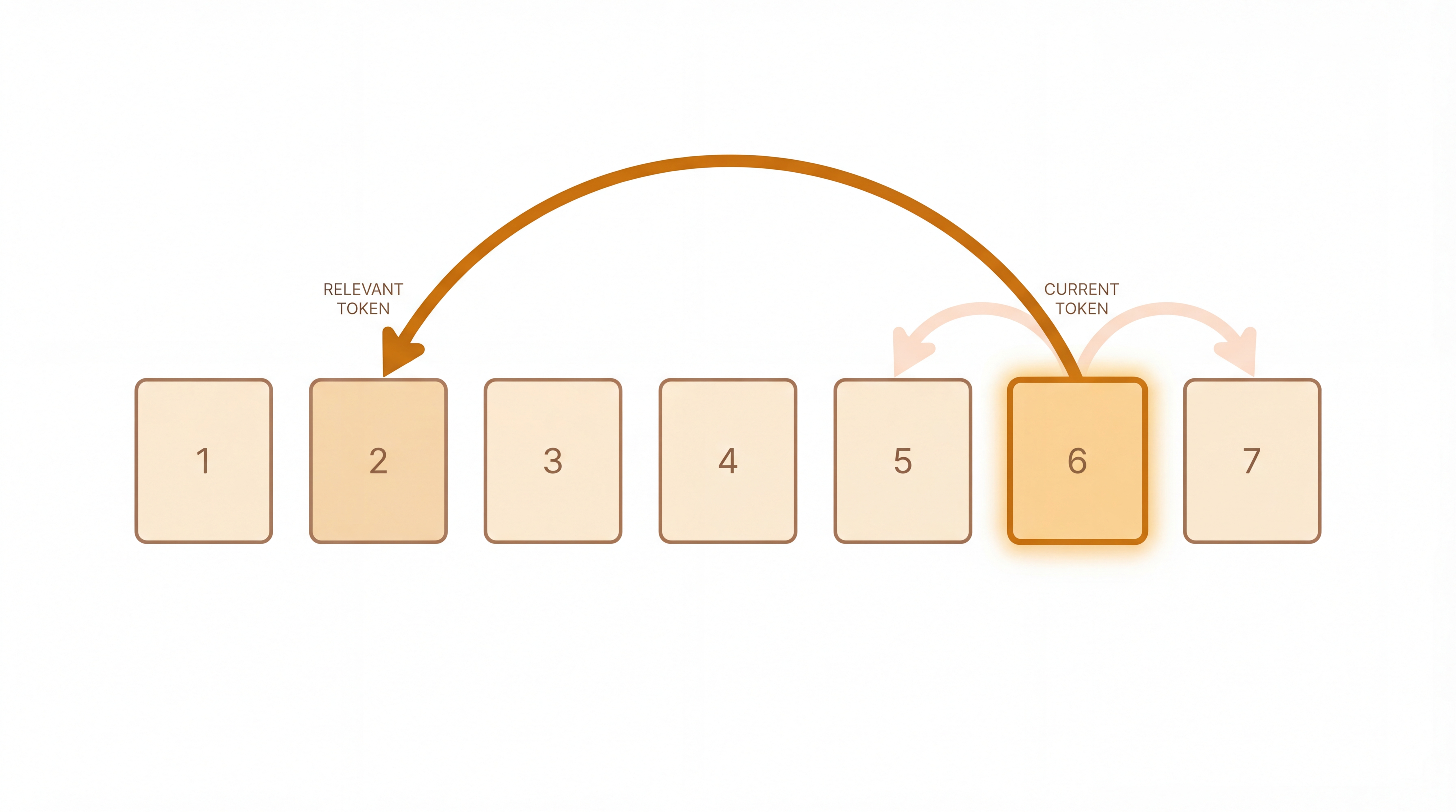
In self-attention, the model looks within the same sequence and decides how strongly each token should attend to every other token. A word can learn to look backward, forward, or even at itself, depending on what helps the task.
Without attention:
current token <- compressed summary of the past

With self-attention:
current token <- weighted combination of all tokens
This is one reason transformers became so powerful. They do not force information through a narrow recurrent chain. They let every token directly compare itself with every other token.
A conceptual self-attention view: the current token can place strong focus on a faraway relevant token instead of relying only on nearby context.
1.1 Processing text data: why this problem is hard
To motivate transformers more concretely, consider a restaurant review like this:
The restaurant refused to serve me a ham sandwich because it only cooks
vegetarian food. In the end, they just gave me two slices of bread.
Their ambiance was just as good as the food and service.
Suppose we want to turn this passage into a representation for a downstream task:
sentiment classification
question answering
review summarization
retrieval or ranking
Three practical problems show up immediately.
First, encoded text can become large very quickly. Even this short passage may contain a few dozen tokens. If each token is represented by a 1024-dimensional embedding, then the network already has to process tens of thousands of input numbers.
For example, with 37 tokens and embedding size 1024:
\[
37 \times 1024 = 37888
\]
So a plain fully connected network is not a natural fit. It does not scale gracefully to longer passages.
Second, text length changes from example to example. One review may be 12 tokens long, another may be 200 tokens long. So we want a mechanism whose parameters do not depend on the exact input length.
This is where parameter sharing becomes important. Just as convolution reuses the same filters at many image positions, self-attention reuses the same projection matrices at every token position.
Third, language contains long-range ambiguity. In the example above, the pronoun "it" refers to the restaurant, not to the ham sandwich. Later, "their" also refers back to the restaurant. A model that only looks locally may miss these relationships.
So the network we want should have three properties:
it should process long inputs efficiently
it should work for variable-length text
it should build input-dependent connections across distant words
That is exactly the setting where self-attention becomes attractive.
Pause and Predict
If a sentence has 20 tokens, how many other tokens can one token directly compare itself with in self-attention?
Answer: All 20 tokens, including itself, because self-attention builds pairwise interactions across the full sequence.
Part 2: The Formal Objective and Definition
Now we can say the goal more precisely.
For each token, self-attention computes a new vector by looking at all tokens in the same sequence and deciding which ones matter more. In other words, self-attention answers this question:
“When updating the representation of this token, how much should I use information from every other token?”
That one sentence already contains the whole idea:
every token starts as a vector,
every token compares itself with all tokens,
every token receives a weighted mixture of information,
and that mixture becomes its new representation.
If you are new to the notation, it helps to keep one concrete picture in mind. Suppose the sentence is:
["The", "cat", "slept"]
When the model updates "slept", it may discover that "cat" matters more than "The". So the new vector for "slept" should contain more information from "cat" than from "The".
The standard form used in transformers follows the scaled dot-product attention introduced in the original Transformer paper by Vaswani et al. (2017):
The symbols look compact, but the logic becomes simple when we read the equation from left to right:
QK^T compares every query with every key.
dividing by sqrt(d_k) keeps those scores numerically stable.
softmax(...) turns the scores into attention weights.
multiplying by V uses those weights to combine value vectors.
So this is not one mysterious operation. It is a short pipeline:
compare -> scale -> normalize -> mix
Before we unpack each symbol, there is one more basic idea to fix in mind:
the input tokens are already vectors called embeddings
attention does not work on raw words like "cat" or "slept"
it works on vector versions of those words
That is why the attention mechanism can be written with matrix operations.
2.1 From a standard neural layer to a self-attention block
A standard neural network layer takes one input vector and returns one output vector. If the input is \(x \in \mathbb{R}^{D}\), a typical layer looks like:
\[
f[x] = \text{ReLU}(\beta + \Omega x)
\]
where:
\(\Omega\) is the weight matrix
\(\beta\) is the bias vector
ReLU is a nonlinearity
This is a useful mental baseline. One vector comes in, one vector goes out.
But a text sequence is not a single vector. It is a collection of token vectors:
\[
x_1, x_2, \ldots, x_N
\]
where each \(x_n \in \mathbb{R}^{D}\).
A self-attention block takes all \(N\) inputs together and returns \(N\) outputs:
Each output corresponds to one token position, but unlike a standard layer, each output may depend on all inputs in the sequence.
So the key shift is:
standard layer: one input vector -> one output vector
self-attention: many input vectors -> many output vectors, each using all inputs
Toy case. If the sequence has three tokens, then the output for token 2 is not computed only from token 2. It can mix information from token 1, token 2, and token 3.
2.2 Computing and weighting values
The textbook-style derivation begins by computing a value vector for each input:
\[
v_m = \beta_v + \Omega_v x_m
\]
Here:
\(x_m\) is the \(m\)th input token vector
\(\Omega_v\) is a shared weight matrix
\(\beta_v\) is a shared bias
\(v_m\) is the value associated with token \(m\)
The important phrase here is shared parameters. The same \(\Omega_v\) and \(\beta_v\) are used for every token in the sequence. This is one reason the method can handle variable-length text.
Now the \(n\)th output is built by taking a weighted sum of all values:
For a fixed token \(n\), all keys compete with one another to explain what the query \(q_n\) needs.
This is why the mechanism is nonlinear overall. The value, key, and query projections are linear, but the attention weights depend on the inputs through:
dot products
exponentials
softmax normalization
Toy case. Suppose one query compares against three keys and produces raw scores:
[1.2, 0.1, 2.0]
After softmax, the third token gets the largest weight, the first token gets a moderate weight, and the second token gets the smallest weight. So the output will be dominated by the third token’s value vector.
2.4 Interpreting Query, Key, and Value
Each input token embedding is first transformed into three different learned views of itself:
Query (Q): What am I looking for?
Key (K): What information do I contain that others may want?
Value (V): What content should be passed along if I am relevant?
That means one token is not represented by just one vector inside attention. It is represented by three role-specific vectors:
one for asking,
one for matching,
one for contributing content.
If token A wants to know whether token B matters, token A’s query is compared with token B’s key. If the match is strong, token B’s value contributes more to token A’s new representation.
This separation is important. A token may be easy to match for one reason but useful to contribute for another. Query, Key, and Value let the model learn those roles separately.
This is similar to a search system:
the query is the search string,
the key is the indexing information attached to each document,
the value is the actual content you retrieve.
Toy case. Imagine the three tokens ["The", "cat", "slept"]. When the model updates the token "slept", its query can be thought of as asking, “Who is performing this action?” The key for "cat" is more likely to match that question than the key for "The", so the value from "cat" contributes more strongly to the new representation of "slept".
You can read that process in plain language like this:
"slept" asks a question
-> "cat" matches that question well
-> "cat" sends more information forward
2.5 Why the dot product?
The term \(QK^T\) computes similarity scores between queries and keys. A larger dot product means stronger alignment between “what this token wants” and “what that token offers.”
If you are new to the dot product, here is the simplest intuition:
if two vectors point in similar directions, the dot product tends to be larger
if they are unrelated, the dot product tends to be smaller
if they oppose each other, it can even become negative
In attention, we use this as a learned similarity test. We are not comparing words directly. We are comparing their learned query and key vectors.
Toy case. Suppose one query is \(q = [2, 1]\). If the key for "cat" is \(k_{cat} = [2, 1]\), then \(q \cdot k_{cat} = 5\). If the key for "The" is \(k_{the} = [0, 1]\), then \(q \cdot k_{the} = 1\). The model will treat "cat" as more relevant than "The" for that query.
This means dot products give us a very compact answer to the question:
“Which tokens match what I need right now?”
2.6 Why divide by \(\sqrt{d_k}\)?
As the key/query dimension \(d_k\) grows, raw dot products tend to grow in magnitude. Large scores can make the softmax output extremely peaked, which leads to unstable learning and weak gradients. Dividing by \(\sqrt{d_k}\) keeps the score scale more controlled.
In beginner language, the scaling factor is a numerical stabilizer. It does not change the logic of attention. It keeps the score values in a range where softmax behaves more smoothly.
Without scaling:
large dimensions can create very large scores,
very large scores can make one token dominate too aggressively,
and learning becomes less stable.
This motivation is emphasized in the Transformer paper and is also discussed in beginner-friendly form in Sebastian Raschka’s walkthrough.
Toy case. Suppose a raw dot-product score is 8 when \(d_k = 4\). After scaling, it becomes \(8 / \sqrt{4} = 4\). If another layer has a raw score 32 when \(d_k = 64\), scaling gives \(32 / \sqrt{64} = 4\) again. The scaling keeps scores from exploding just because the vector dimension is larger.
So the question is not “Why make the score smaller?” The better question is:
“Why keep score magnitudes comparable as vector size changes?”
That is what the scaling term does.
2.7 What does softmax do?
Softmax converts each row of scores into a probability-like distribution:
every value becomes non-negative,
each row sums to 1,
larger scores receive larger weights.
So after softmax, each token has a learned weighting over all tokens in the sequence.
This step is what turns raw similarity numbers into something operational. Before softmax, scores are just arbitrary real values. After softmax, they become attention weights that tell the model how much each token should matter.
Another useful intuition is that softmax creates competition within a row. If one token’s score rises a lot, the others usually get less weight in that same row.
Toy case. If one token produces scores [2, 1, 0] over three tokens, softmax turns them into approximately [0.67, 0.24, 0.09]. The first token gets most of the attention, the second gets some, and the third gets very little.
That row can now be read in plain English:
pay a lot of attention to token 1
pay some attention to token 2
pay little attention to token 3
2.8 What is the final output?
The attention weights are multiplied by the value matrix \(V\). This produces a new representation for every token:
each output token is a weighted sum of value vectors,
the weights depend on relevance,
relevance is learned through the query-key comparisons.
This is the step where attention actually moves information.
Up to now, the model has only answered:
“Where should I look?”
Now it answers:
“What information should I bring back from those places?”
That is why the value vectors matter so much. The attention weights tell us how strongly to use each token, and the values provide the content to combine.
Toy case. Suppose the attention weights for one token are [0.7, 0.2, 0.1], and the three value vectors are \(v_1 = [2, 0]\), \(v_2 = [0, 2]\), and \(v_3 = [1, 1]\). Then the output becomes:
So the output is not copied from one token. It is a weighted blend of several value vectors.
That is the full mechanism.
If you want one sentence to remember this entire section, use this:
self-attention compares tokens with queries and keys, turns those comparisons into weights, and uses the weights to mix value vectors into a new representation.
And if you want one tiny workflow to hold in your head before moving to the matrix version, it is this:
token embeddings
-> Q, K, V
-> similarity scores
-> softmax weights
-> weighted sum of values
-> new token representations
A clean summary of the formal self-attention pipeline: compare queries and keys, scale the scores, normalize them with softmax, and mix values into the final output.
2.9 Self-attention summary
At this point, we can summarize self-attention in a more textbook-aligned way.
For each token position:
compute a value vector with a shared linear transformation
compute a query vector for the current token
compute key vectors for all tokens
compare the current query with all keys
normalize those comparisons into attention weights
take a weighted sum of the values
This mechanism satisfies the requirements we identified in the text-processing example:
the same parameters are reused across token positions
the method works for different sequence lengths
each output can connect to distant tokens
the strength of those connections depends on the input itself
So self-attention is not just a convenient formula. It is a way to build shared, input-dependent interactions across a sequence.
Shape Check
If \(Q \in \mathbb{R}^{n \times d_k}\) and \(K \in \mathbb{R}^{n \times d_k}\), what is the shape of \(QK^T\)?
Answer:\([n, n]\). Each row corresponds to one query token comparing itself with all key tokens.
Part 3: Step-by-Step Mathematical Walkthrough with Matrices
Let the input sequence contain \(n\) tokens, and let each token embedding have dimension \(d_{model}\).
We arrange the embeddings row-wise into a matrix:
\[
X \in \mathbb{R}^{n \times d_{model}}
\]
Each row is one token vector.
3.1 Token embeddings
X = [x_1
     x_2
     ...
     x_n]            shape: [n, d_model]
These embeddings are the model’s starting description of the tokens.
\[
A = \text{softmax}(\hat{S}) \in \mathbb{R}^{n \times n}
\]
Each row of \(A\) sums to 1. Row \(i\) gives the attention distribution for token \(i\).
3.5 Aggregate values
Finally:
\[
O = AV \in \mathbb{R}^{n \times d_v}
\]
Each output row is a weighted combination of all value vectors.
3.6 The whole pipeline in one shape diagram
Input embeddings:
X                      [n, d_model]

Linear projections:
Q = X W_Q              [n, d_k]
K = X W_K              [n, d_k]
V = X W_V              [n, d_v]

Similarity scores:
Q K^T                  [n, n]

Scaled scores:
(Q K^T) / sqrt(d_k)    [n, n]

Attention weights:
softmax(...)           [n, n]

Context vectors:
softmax(...) V         [n, d_v]
At this point, self-attention should feel less mysterious. It is just a sequence of matrix multiplications with a normalization step in the middle.
A conceptual pipeline for self-attention: input embeddings are projected into Q, K, and V, used to form scores, normalized by softmax, and then combined into output representations.
Think Like the Model
Suppose token 3 gives a very large score only to token 1 and very small scores to every other token. After softmax, what happens?
Answer: The row for token 3 becomes concentrated on token 1, so token 3’s new representation is dominated by token 1’s value vector.
3.7 Textbook matrix form and notation conventions
So far, this tutorial has stacked token vectors as rows:
\[
X \in \mathbb{R}^{N \times D}
\]
That is a very common implementation view in code. But many textbooks, including the one you referenced, stack token vectors as columns:
\[
X \in \mathbb{R}^{D \times N}
\]
Both conventions describe the same computation. They only differ in where the token dimension is placed.
In the column-wise textbook convention, the value, query, and key matrices are written as:
\[
V[X] = \beta_v \mathbf{1}^T + \Omega_v X
\]
\[
Q[X] = \beta_q \mathbf{1}^T + \Omega_q X
\]
\[
K[X] = \beta_k \mathbf{1}^T + \Omega_k X
\]
where:
\(X \in \mathbb{R}^{D \times N}\)
\(\mathbf{1} \in \mathbb{R}^{N \times 1}\) is a vector of ones
each column is one token representation
The self-attention computation can then be written as:
but the two formulas describe the same algorithm under different matrix layout choices.
The important lesson is this:
row-wise notation is often easier for implementation
column-wise notation is often convenient for textbook derivations
If you understand one, you can translate to the other by tracking where the token dimension lives.
3.8 Positional encoding: what self-attention alone misses
Self-attention has one major blind spot: by itself, it does not know the order of tokens.
If you reorder the input tokens and apply the same reorder to the embeddings, self-attention will reorder its outputs in the same way. In other words, the mechanism is permutation equivariant.
That is a problem for language because:
The woman ate the raccoon.
The raccoon ate the woman.
These sentences contain almost the same words, but their meanings are very different because the order is different.
So real transformers add position information explicitly.
Absolute positional encodings
The simplest idea is to add a position vector to each token embedding:
\[
\tilde{X} = X + P
\]
where:
\(X\) contains token embeddings
\(P\) contains position encodings
each row or column of \(P\) is different depending on position
These positional encodings can be:
fixed, such as sinusoidal encodings
learned, where the model trains a separate position embedding for each location
In plain language, absolute positional encoding tells the model:
this token is in position 1
this token is in position 2
this token is in position 3
Relative positional encodings
Sometimes the exact absolute position matters less than the distance between two tokens.
For example, in language, the fact that one word is:
one token to the left
three tokens to the right
far away in the sentence
may matter more than whether it appears at absolute position 17 or 42.
Relative positional encodings inject information about offsets between tokens, often by modifying the attention scores. A simple conceptual form is:
where \(b_{i-j}\) is a learned bias that depends on the relative distance between positions \(i\) and \(j\).
Why this matters in practice
Without positional information:
repeated identical tokens can become hard to distinguish
word order can be lost
sentence meaning can collapse into something more like a bag of token vectors
That is why almost all practical transformer models combine self-attention with some form of positional encoding.
For clarity, the toy PyTorch examples in this article omit positional encodings. That keeps the attention mechanism easy to inspect. But real transformer models almost always include them.
Part 4: A Small Working PyTorch Example
The math becomes much easier to trust once you can see actual tensor shapes.
4.1 Start with embeddings
The following snippet is intentionally small. It creates an embedding table with 6 possible token IDs, where each token is mapped to a 16-dimensional vector.
torch.manual_seed(123) fixes the random seed so the embedding values are reproducible.
torch.nn.Embedding(6, 16) creates a learnable lookup table with:
6 rows, one for each token ID from 0 to 5
16 columns, so every token becomes a 16-dimensional vector
sentence_int = torch.tensor([0, 1, 2, 3]) defines a sequence of 4 token IDs.
embed(sentence_int) looks up the corresponding rows in the embedding table.
.detach() removes the tensor from gradient tracking so we can inspect it as a fixed example.
The printed shape is:
\[
[4, 16]
\]
Why?
there are 4 tokens in sentence_int,
each token becomes a 16-dimensional vector.
So the output contains one row per token and one column per embedding feature.
This matrix is exactly what we called \(X\) in the mathematical walkthrough:
\[
X \in \mathbb{R}^{4 \times 16}
\]
That means:
\(n = 4\)
\(d_{model} = 16\)
4.2 Why embeddings matter
An embedding layer turns discrete token IDs into dense vectors that a neural network can work with. Token IDs by themselves have no geometry. The fact that token 4 is numerically larger than token 1 does not mean it is semantically larger. Embeddings fix that by mapping tokens into a learned continuous space where similarity can be represented.
Self-attention does not work directly on token IDs. It works on the embedding matrix.
Pause and Predict
If the sentence had 10 tokens and the embedding size were 64, what would the embedding output shape be?
Answer:[10, 64].
4.3 Extend the example to self-attention
Now let us build a very small self-attention computation from the embedding output.
Q shape: torch.Size([4, 8])
K shape: torch.Size([4, 8])
V shape: torch.Size([4, 8])
Conceptually, this implements:
\[
Q = XW_Q, \quad K = XW_K, \quad V = XW_V
\]
with:
\(X \in \mathbb{R}^{4 \times 16}\)
\(W_Q, W_K, W_V \in \mathbb{R}^{16 \times 8}\)
\(Q, K, V \in \mathbb{R}^{4 \times 8}\)
One implementation detail is worth noting. In matrix notation, we usually write \(XW_Q\). In PyTorch, nn.Linear(16, 8) stores its weight with shape [8, 16] and applies the corresponding multiplication internally. So the math and the code are saying the same thing even though the stored parameter layout looks transposed.
4.4 Compute attention scores, weights, and outputs
softmax(..., dim=-1) turns each row into attention weights.
attention_weights @ V computes the weighted mixture of value vectors.
Now the shapes should make immediate sense:
scores: [4, 4]
attention_weights: [4, 4]
context: [4, 8]
The matrix [4, 4] is important. It means:
4 query tokens,
each query token looks at 4 key tokens.
Each row of attention_weights sums to 1, which is why the printed row sums are all 1.
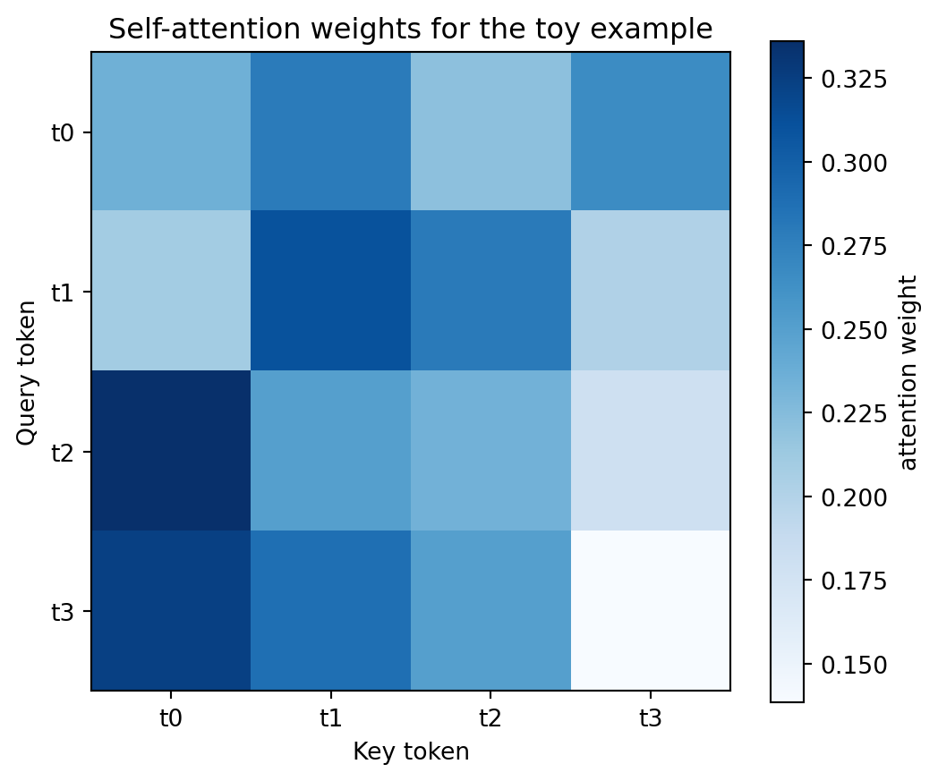
4.5 A simple attention heatmap
import matplotlib.pyplot as pltplt.figure(figsize=(6, 5))plt.imshow(attention_weights.detach().numpy(), cmap="Blues")plt.colorbar(label="attention weight")plt.xticks(range(4), [f"t{i}"for i inrange(4)])plt.yticks(range(4), [f"t{i}"for i inrange(4)])plt.xlabel("Key token")plt.ylabel("Query token")plt.title("Self-attention weights for the toy example")plt.show()
Read this heatmap row by row. A darker cell means the query token on that row is placing more weight on the key token in that column.
This is the most useful mental model for attention:
rows ask the question,
columns offer information,
cell brightness shows how much information flows.
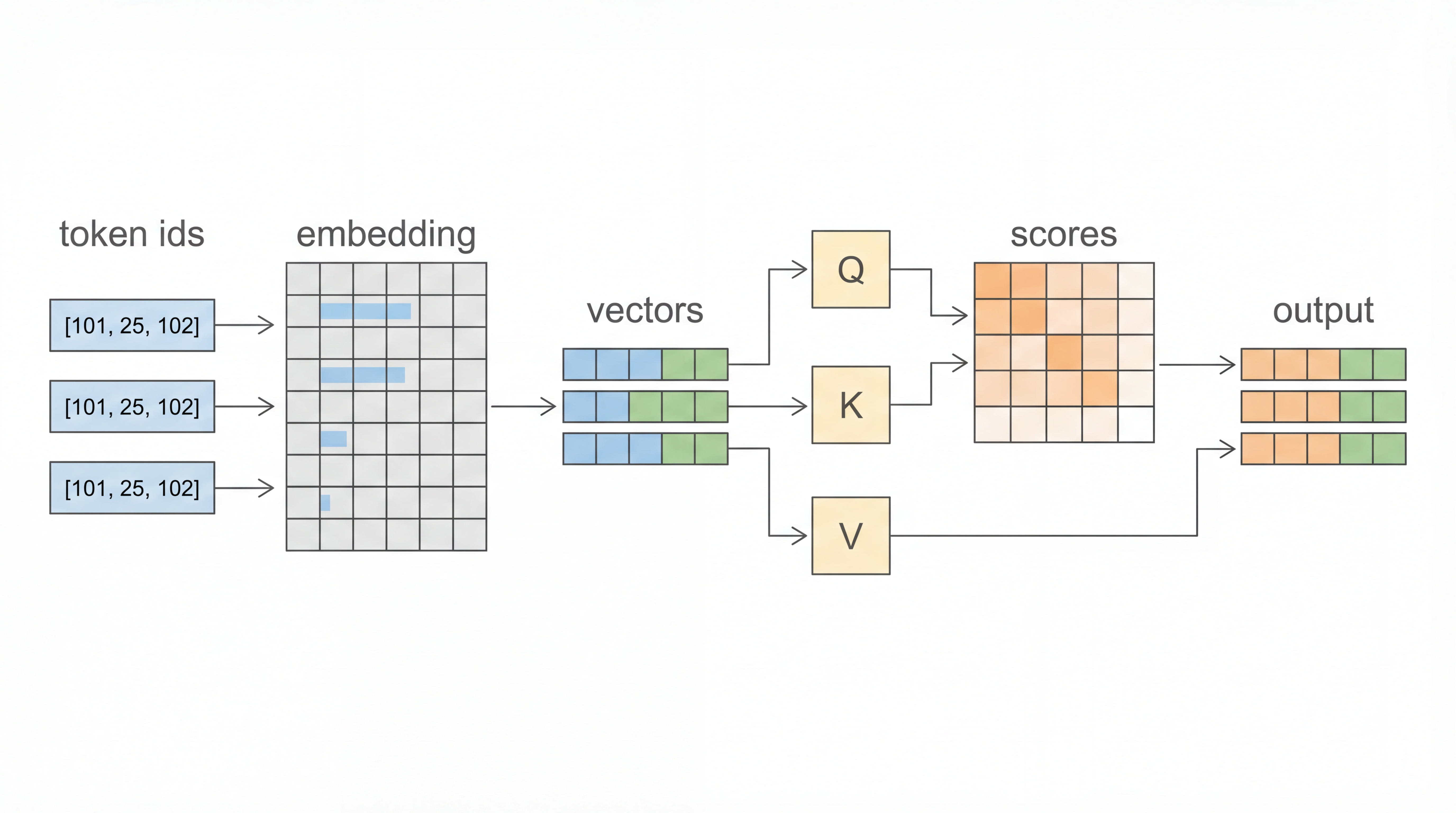
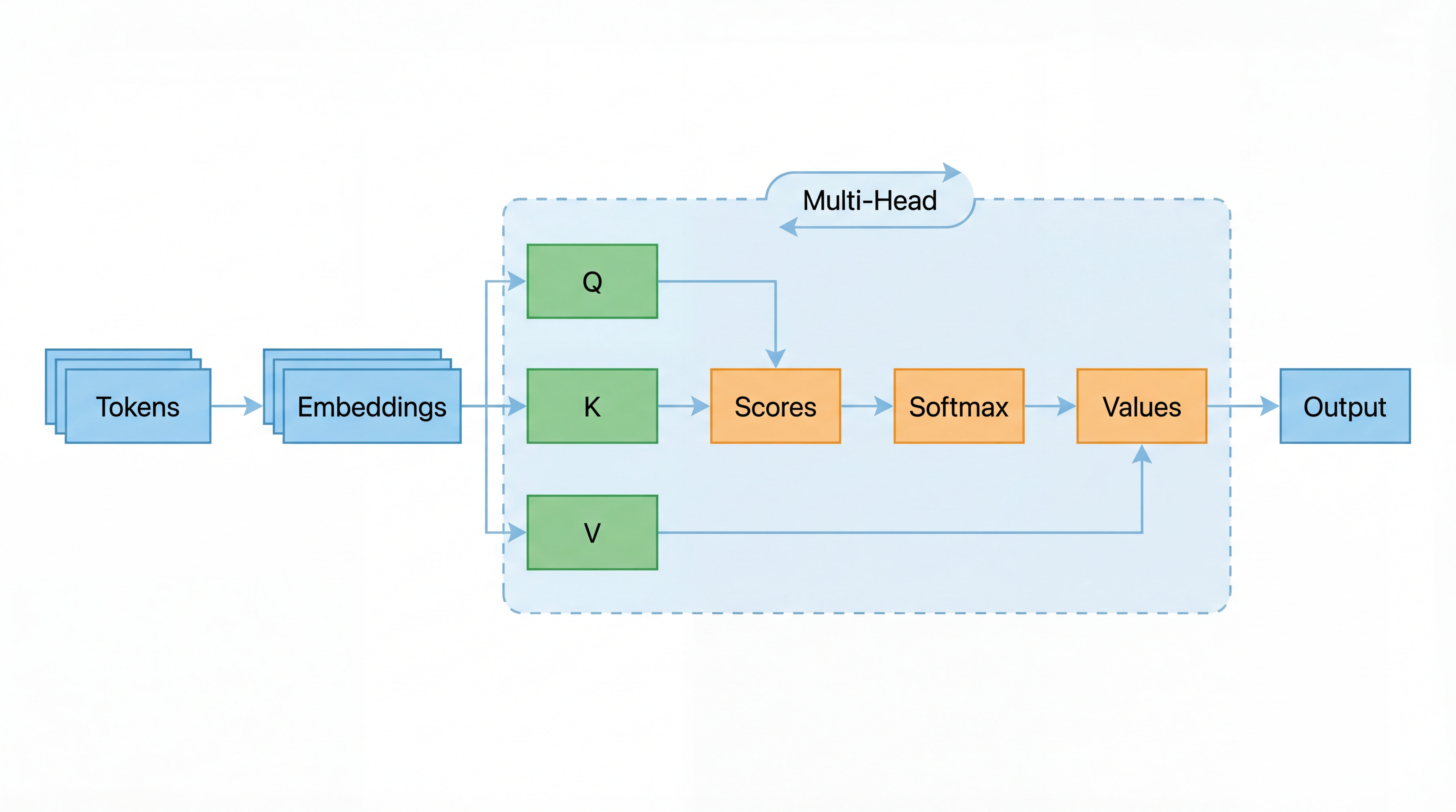
A white-background summary of the code path from token ids to embeddings, then to Q, K, V, scores, and output vectors.
Part 5: From Single-Head Attention to Multi-Head Attention
At this point, you might wonder: if one attention map is useful, why not stop there?
The answer is that one head has only one way of looking at the sequence at a time.
A sentence often contains several kinds of relationships simultaneously:
grammatical relationships
semantic similarity
long-range references
local phrase structure
One attention head might learn subject-verb agreement. Another might learn modifier relationships. Another might focus on nearby context. A single head can represent only one weighted view per layer. Multi-head attention gives the model multiple learned views in parallel.
5.1 The idea of multiple heads
Instead of using one set of projections, we create several smaller sets:
X [n, d_model]
  -> head 1 attention -> [n, d_head]
  -> head 2 attention -> [n, d_head]
  -> ...
  -> head h attention -> [n, d_head]

concatenate all heads -> [n, h * d_head] = [n, d_model]
final linear projection -> [n, d_model]
If d_model = 16 and num_heads = 4, then each head can use:
\[
d_{head} = 16 / 4 = 4
\]
Each head gets a smaller subspace, but the model gains several parallel ways to compare tokens.
5.2 The multi-head attention formula
The standard formulation from the Transformer paper is:
A conceptual multi-head attention diagram: the input is split across several heads, each head computes its own attention pattern, and the resulting representations are concatenated and projected.
5.3 Why concatenation and output projection matter
Two details in multi-head attention are easy to miss:
why we split the model dimension into several smaller heads
why we concatenate the head outputs and then apply one more matrix \(W_O\)
Then each head only works in a 4-dimensional subspace. That sounds smaller, but it is exactly the point. Each head gets to build its own similarity function in its own learned feature space.
One head may care about local phrase structure:
"the red car"
Another head may care about a long-distance relation:
mixes information across heads. Without this final step, the heads would simply sit side by side. The output projection lets the model combine them into a richer shared representation.
Toy case. Imagine:
Head 1 focuses on subject information
Head 2 focuses on verb agreement
Head 3 focuses on nearby modifiers
Head 4 focuses on long-range references
Concatenation stacks those four views together, and the output projection learns how to merge them into one final token embedding.
x is the same tensor used for queries, keys, and values, so this is self-attention
batch_first=True means the input shape is [batch, tokens, d_model]
attn_output has shape [1, 4, 16]
attn_weights has shape [1, 4, 4, 4]
That last shape means:
batch size = 1
number of heads = 4
4 query tokens
4 key tokens
So PyTorch is giving you the per-head attention maps directly.
If you only want the output tensor and do not care about each head’s weight matrix, you can call the module without inspecting attn_weights.
Why this example matters. The manual implementation helps you understand the mechanics. The built-in module helps you work with real models.
5.6 Why multiple heads help
Multi-head attention is powerful because it lets the model distribute its reasoning. Instead of forcing one attention map to capture every useful relationship, the model learns several complementary attention patterns.
A practical way to think about it is this:
one head can learn who modifies whom
another can learn what refers to what
another can learn which nearby tokens form a phrase
another can learn what global context matters
That is why one head is often insufficient.
Pause and Predict
If d_model = 24 and num_heads = 6, what is d_head?
Answer:4, because each head gets 24 / 6 features.
Part 6: Conceptual Checkpoints That Build Intuition
This section is not new content. It is a way to test whether the flow so far is holding together.
Checkpoint 1: What happens if two tokens have nearly identical keys?
Then any query that matches one of them may also match the other strongly. Their columns in the attention score matrix can become similar, which means they may receive similar attention weights.
Checkpoint 2: What happens if one score in a row becomes much larger than the rest?
Softmax will concentrate most of the probability mass on that one position. The output for that query token will be dominated by the corresponding value vector.
Checkpoint 3: Why not skip the value matrix and use keys directly?
Because keys are used for matching, not for content transport. The model benefits from separating:
how to compare tokens (Q and K)
what information to pass forward (V)
That separation gives the mechanism more flexibility.
Checkpoint 4: Why is self-attention called “self” attention?
Because the queries, keys, and values all come from the same input sequence. In cross-attention, the queries come from one sequence and the keys/values come from another.
Checkpoint 5: What happens if all scores in one row are equal?
Then softmax turns that row into a uniform distribution. If there are \(n\) tokens, each one gets weight \(1/n\).
That means the output for that query token becomes a simple average of the value vectors rather than a selective focus on a few tokens.
Checkpoint 6: What happens if the attention weights stay the same but the value vectors change?
Then the model still looks at the same positions, but it retrieves different content from them.
This is an important distinction:
queries and keys decide where to look
values decide what information is brought back
So attention location and transported content are related, but they are not the same thing.
Checkpoint 7: What happens when a mask blocks a token?
Its score is effectively pushed to a very large negative number before softmax. After softmax, that token receives probability very close to zero.
So masking does not merely “discourage” attention. It removes that position from consideration for that row.
Checkpoint 8: Can two different heads attend to the same token?
Yes. Multi-head attention does not force heads to focus on different places. Two heads can look at the same token but still use it differently because their projections are different.
For example, two heads may both attend strongly to the same noun:
one head may care about grammatical number
another may care about semantic identity
The attended position can be the same even when the learned function is different.
Checkpoint 9: What happens if two tokens have identical embeddings and there is no positional information?
Then the attention mechanism has no built-in reason to distinguish them. Their queries, keys, and values may become identical, which makes their behavior symmetric.
This is one reason positional encoding is essential in transformers. It gives the model a way to distinguish “same word, different place.”
Checkpoint 10: What happens if d_model is not divisible by the number of heads?
In the standard implementation, you cannot split the model dimension evenly across heads. That is why most implementations require:
\[
d_{model} \bmod h = 0
\]
For example, d_model = 16 works with num_heads = 4, but not with num_heads = 3 in the usual equal-sized head design.
Checkpoint 11: What happens if a query vector is close to zero?
Then its dot products with all keys may become very similar. If the scores are nearly equal, the softmax row becomes close to uniform, and the output becomes close to an average of value vectors.
So a weak or non-informative query leads to broad, less selective attention.
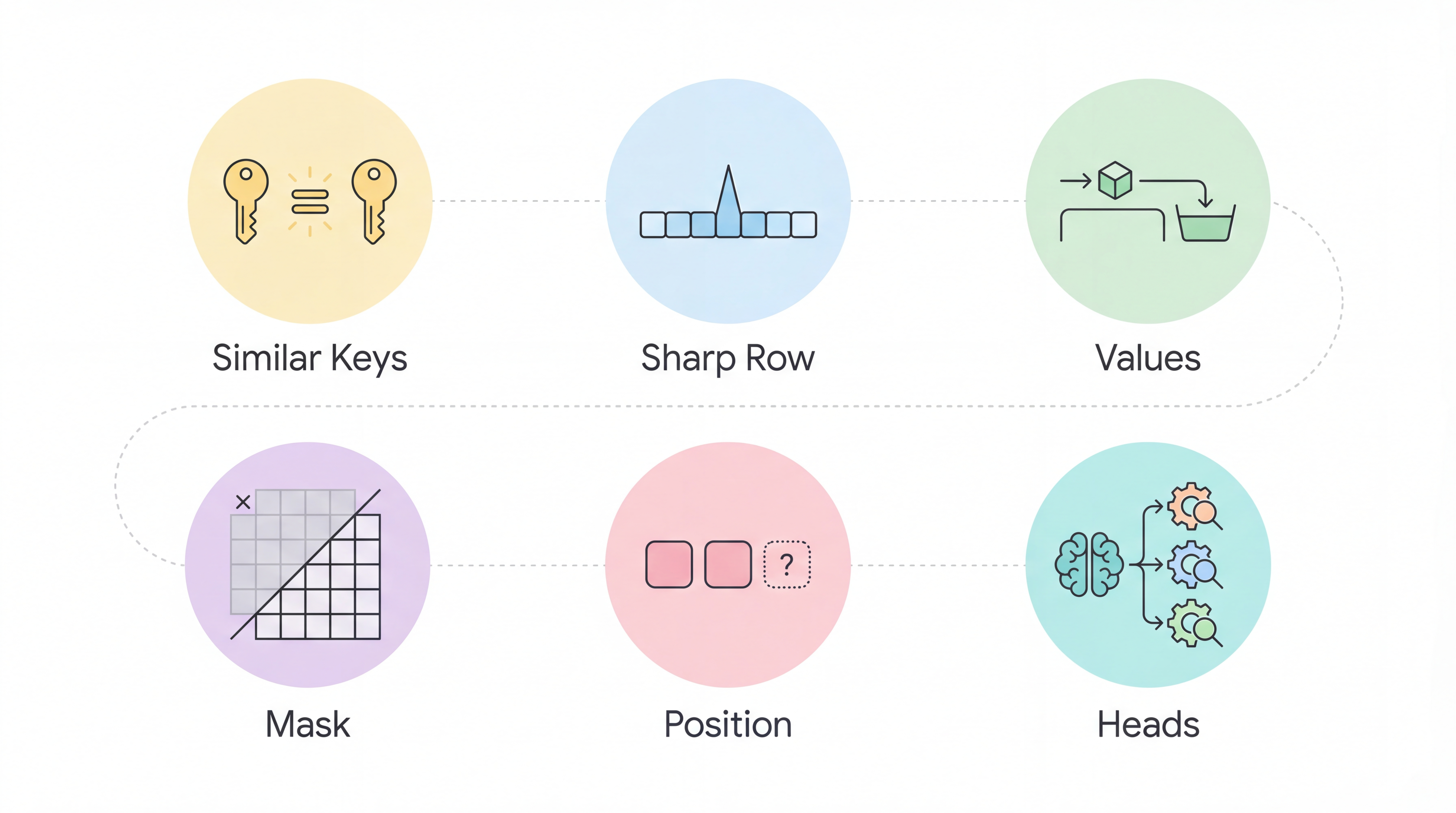
A conceptual map of the main intuition checks for attention: similar keys, sharp softmax rows, value transport, masking, positional information, and head specialization.
Part 7: Where Self-Attention and Multi-Head Attention Are Used
Once you understand the mechanism, many modern architectures become easier to read.
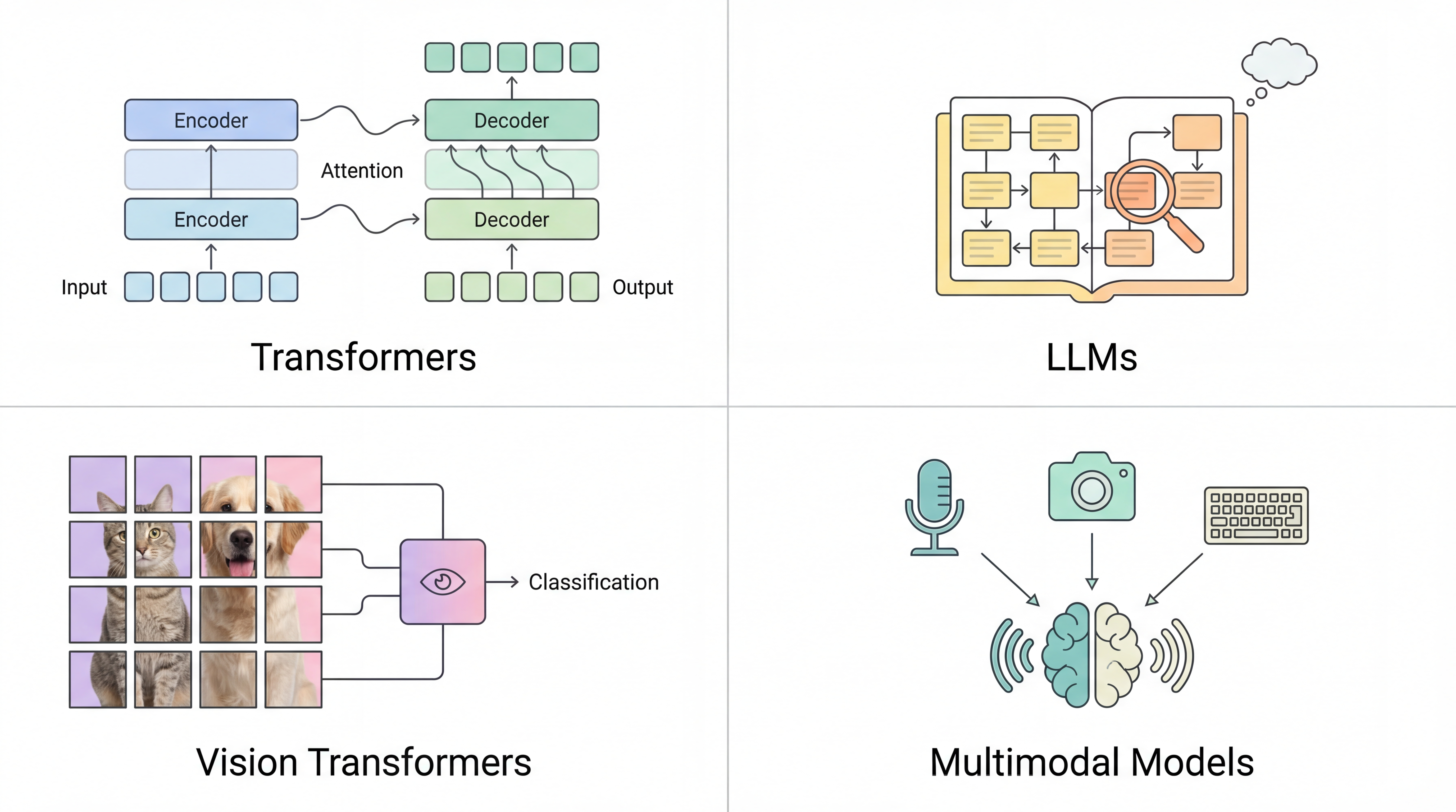
7.1 Transformers
Transformers are built around stacked attention and feed-forward blocks. In encoder layers, self-attention lets every token gather context from the full sentence. In decoder layers, masked self-attention lets each token look only at previous tokens during generation.
7.2 Large Language Models
LLMs rely on attention to decide which earlier tokens matter for predicting the next token. This is why a model can relate a pronoun to an earlier noun, maintain topic continuity, or use instructions given many tokens earlier in the prompt.
7.3 Vision Transformers
In a Vision Transformer, the “tokens” are image patches rather than words. Self-attention lets one patch compare itself with all other patches, which helps the model reason about global spatial structure.
7.4 Multimodal Models
In multimodal models, attention helps connect information across modalities such as text and images. Self-attention may operate within one modality, while cross-attention may connect one modality to another. The same basic idea scales across language, vision, speech, and mixed-input systems.
A white-background overview of major attention applications across Transformers, LLMs, Vision Transformers, and multimodal models.
Part 8: Interview Questions
Attention is a common interview topic because it tests whether you can move between intuition, equations, tensor shapes, and implementation details.
Open each dropdown and try answering first before reading the solution. The goal here is not just recall. It is to practice moving between definition, math, and implementation.
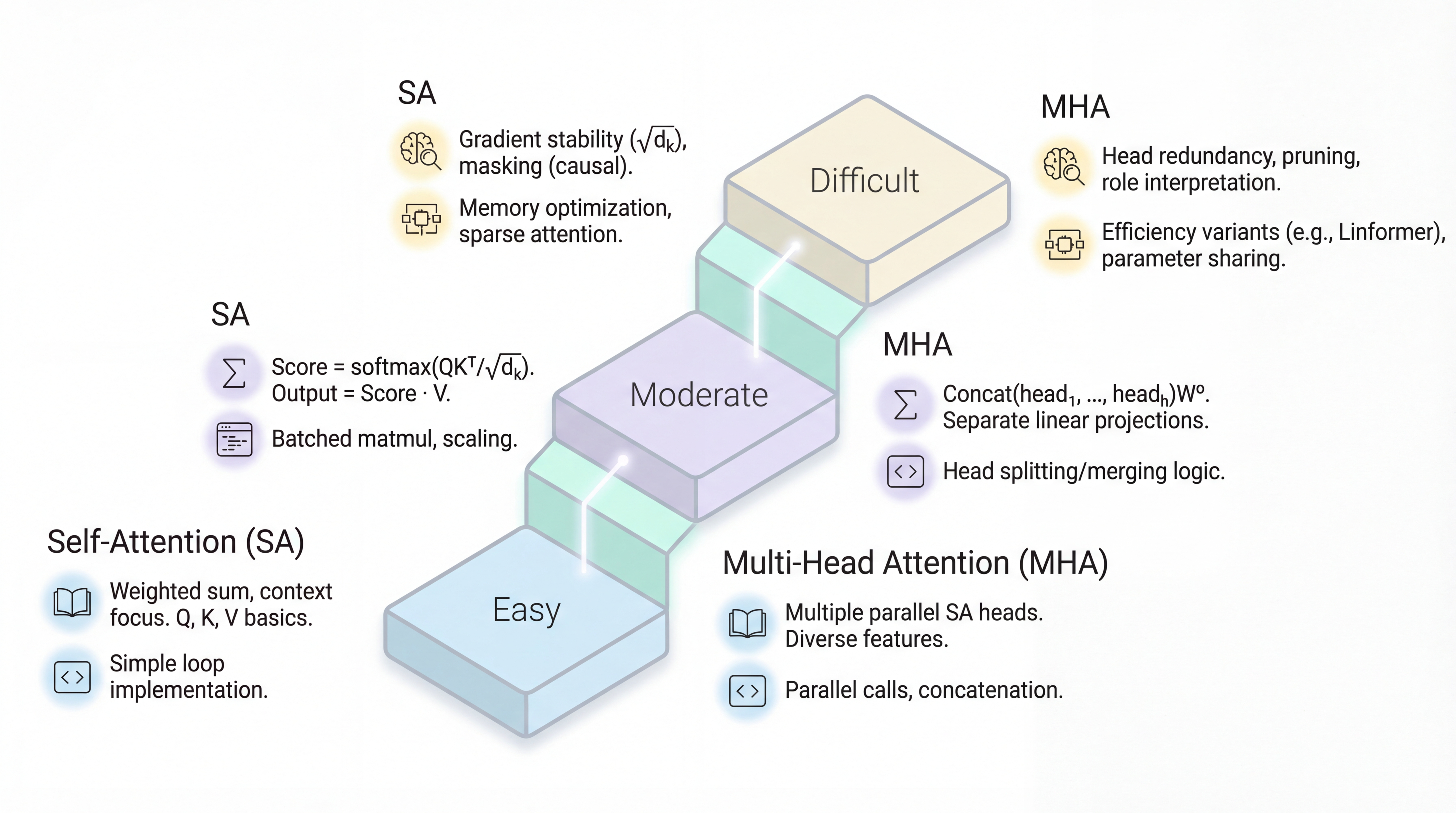
Easy
Easy 1. What problem does self-attention solve compared with plain RNNs?
Answer. Self-attention gives each token direct access to every other token in the sequence. That makes long-range dependencies easier to learn because information does not have to travel through a long recurrent chain.
Definition. In self-attention, each token builds a new representation by taking a weighted combination of all tokens in the same sequence.
Easy 2. In one sentence, what do Query, Key, and Value represent?
Answer.
Query: what this token is looking for
Key: what this token offers for matching
Value: what information this token contributes if selected
That is why the model uses queries and keys for comparison, then values for aggregation.
Easy 3. Why does the attention score matrix have shape [n, n]?
Answer. If there are n tokens, each of the n query vectors compares itself against all n key vectors. So we get one score for every query-key pair.
Rows correspond to query tokens and columns correspond to key tokens.
Easy 4. What does softmax do in self-attention?
Answer. Softmax converts raw attention scores into normalized weights:
all weights become non-negative,
each row sums to 1,
larger scores receive larger weights.
So softmax turns similarity scores into a usable weighting distribution over tokens.
Easy 5. Why does an embedding layer output shape [4, 16] for 4 tokens with embedding size 16?
Answer. Because there are 4 input token IDs, and each token is mapped to a vector of length 16.
Definition. An embedding layer is a learnable lookup table that maps discrete token IDs to dense vectors.
Easy 6. What is the difference between self-attention and cross-attention?
Answer.
In self-attention, queries, keys, and values all come from the same sequence.
In cross-attention, queries come from one sequence, while keys and values come from another.
Example: a decoder in a translation model may use cross-attention to look at encoder outputs.
Easy 7. Why do transformers use multiple heads instead of one?
Answer. Multiple heads let the model learn several different token relationships at the same time. One head may focus on syntax, another on coreference, another on local context, and another on long-range structure.
Definition. Multi-head attention is parallel self-attention performed in multiple learned subspaces, followed by concatenation and an output projection.
Moderate
Moderate 1. Derive the shapes of Q, K, V, QK^T, and AV when X ∈ R^{n × d_model}.
Moderate 2. Why do we divide attention scores by sqrt(d_k)?
Answer. Because raw dot products grow in magnitude as the key/query dimension grows. If the scores become too large, softmax becomes too sharp and gradients become less stable.
Math intuition. If vector components are roughly unit scale, then the dot product magnitude tends to grow with dimension. Scaling by
\[
\frac{1}{\sqrt{d_k}}
\]
keeps the score distribution better behaved.
Moderate 3. Compute the output if the attention weights are [0.6, 0.3, 0.1] and the value vectors are [1, 0], [0, 2], and [3, 1].
Answer.
The output is the weighted sum:
\[
0.6[1,0] + 0.3[0,2] + 0.1[3,1]
\]
\[
= [0.6,0] + [0,0.6] + [0.3,0.1]
\]
\[
= [0.9, 0.7]
\]
This is the core idea of attention: the output is a blend, not a hard selection.
Moderate 4. What is the computational complexity of self-attention with sequence length n?
Answer. The dominant cost comes from the token-to-token interaction matrix.
Math.
Computing scores QK^T is roughly O(n^2 d_k)
Multiplying attention weights by V is roughly O(n^2 d_v)
In practice, this is commonly summarized as quadratic in sequence length:
\[
O(n^2 d)
\]
That quadratic dependence on n is why long-context modeling is expensive.
Moderate 5. How does causal masking work in decoder self-attention?
Answer. Causal masking prevents a token from attending to future tokens. Before softmax, the model adds a large negative value such as -inf to disallowed positions.
where M is 0 for allowed positions and -inf for masked future positions.
After softmax, future-token probabilities become effectively zero.
Moderate 6. In PyTorch, why does nn.Linear(16, 8) conceptually match multiplication by a matrix of shape [16, 8] even though the stored weight is [8, 16]?
Answer.nn.Linear(in_features, out_features) stores weights as [out_features, in_features] because of how the internal computation is implemented. But conceptually, the layer maps a vector in R^{16} to a vector in R^{8}, which matches multiplication by a conceptual projection matrix of shape [16, 8].
So the math view and the implementation view are consistent; they just store the weight in transposed form.
Moderate 7. Write the minimal PyTorch code for single-head scaled dot-product attention.
Difficult 1. Why does self-attention need positional information?
Answer. Plain self-attention compares token content, but by itself it does not encode order. If you permute the token sequence and permute the embeddings the same way, the attention operation changes accordingly but does not know which token came first unless you inject positional information.
Key idea. Positional embeddings or positional encodings break this symmetry so "dog bites man" and "man bites dog" are no longer treated as the same bag of token vectors.
Difficult 2. What kinds of information might different heads learn, and why can some heads become redundant?
Answer. Different heads can specialize in syntax, local context, delimiter tracking, coreference, or long-range dependencies. But in practice, some heads learn overlapping patterns. Once several heads discover similar useful structures, later heads may contribute less unique information.
That is why pruning studies sometimes find that removing a subset of heads causes only a small performance drop.
Difficult 3. Are attention weights good explanations of model behavior?
Answer. They can be useful diagnostic signals, but they are not guaranteed to be causal explanations.
Reason. A token may receive high attention weight and still not be the true reason for the final model decision, because the output also depends on value vectors, residual connections, layer stacking, MLP blocks, and later transformations.
So attention can be interpretable, but interpretability is weaker than causality.
Difficult 4. What would change if softmax were replaced by another normalization such as sparsemax or sigmoid gating?
Answer. The behavior of the attention distribution would change.
Softmax: dense distribution, sums to 1, strongly competitive
Sparsemax: can produce exact zeros, giving sparse attention
Sigmoid gating: weights are independent rather than forced to compete in a row-wise distribution
So replacing softmax changes smoothness, sparsity, competition among tokens, and often optimization behavior.
Difficult 5. How does grouped-query or multi-query attention reduce inference cost?
Answer. In standard multi-head attention, each head has its own queries, keys, and values. In grouped-query attention or multi-query attention, many query heads share fewer key and value heads.
Why this helps. During autoregressive decoding, keys and values are cached. Sharing K/V heads reduces the KV-cache size and the memory bandwidth needed at inference time, which is especially useful in large language models.
Difficult 6. How would you modify the basic attention pipeline to support padding masks?
Answer. Add a mask before softmax so padded positions cannot receive attention probability.
This ensures the model ignores padding tokens when forming context.
Difficult 7. What happens if two tokens have identical embeddings and there is no positional information?
Answer. Then their projected queries, keys, and values will also be identical if the same linear layers are applied. That means self-attention has no basis for distinguishing them.
Implication. Without positional information or other distinguishing context, the model treats those tokens symmetrically. This is one more way to see why positional encoding is essential.
A light interview roadmap for self-attention and multi-head attention, moving from easy definitions to moderate math/code and difficult systems-level reasoning.
Part 9: Closing the Loop
The most important lesson is that self-attention is not just a formula to memorize. It is a sequence of very concrete operations:
turn tokens into vectors,
project them into queries, keys, and values,
compare queries with keys,
normalize the scores,
mix values using those normalized weights.
Multi-head attention repeats that idea in several subspaces at once.
If you can explain those five steps clearly and track the shapes at each stage, you already understand the core engine behind transformers.
A final white-background summary loop linking tokens, embeddings, QKV projections, scores, softmax, value mixing, and multi-head output.
A practical study strategy
If you want this topic to really stick, try the following order:
Re-run the toy code cells and verify the shapes without looking.
Change the number of tokens and embedding size, then predict the new shapes first.
Change num_heads and compute d_head manually before running the multi-head example.
Only after that move on to reading full transformer implementations.
References
This article draws on the formal transformer definition from Attention Is All You Need and uses a student-friendly, code-first teaching style inspired by the following resources: