Why Should You Care?

Every machine-learning model that touches geographic coordinates (species distribution models, climate emulators, satellite image classifiers, epidemiological forecasters) faces the same quiet assumption: that latitude and longitude behave like \(x\) and \(y\) on a flat sheet of paper.

They do not. Earth is a sphere.

Near the equator the approximation is tolerable. But walk toward the North Pole and something strange happens: lines of longitude, which looked comfortably parallel on your flat map, rush together and collapse into a single point. A model that still thinks it is working on a rectangle will hallucinate boundaries, smear predictions, and produce artifacts exactly where climate scientists care most: the rapidly changing polar regions.

This paper asks a deceptively simple question: what if the positional encoding respected the sphere from the start?

The answer turns out to be Spherical Harmonics, a family of basis functions that physicists have used for two centuries to describe gravity fields, planetary magnetospheres, and electron orbitals. Combined with Sinusoidal Representation Networks (SirenNets), the result is a location encoder that is mathematically principled, empirically dominant across four benchmarks, free of polar artifacts, and computationally practical.

Let us see how it works.

The Location Encoding Framework

Across the literature on geographic ML, location encoders follow a two-stage template:

\[ y = \underbrace{\text{NN}}_{\text{neural network}}\!\Big(\underbrace{\text{PE}(\lambda, \phi)}_{\text{positional embedding}}\Big) \]

Raw coordinates (longitude \(\lambda \in [-\pi,\pi]\) and latitude \(\phi \in [-\pi/2,\pi/2]\)) first pass through a non-parametric positional embedding (PE) that lifts them into a higher-dimensional feature space. A small neural network (NN) then maps these features to the task output: a classification logit, a regression target, or a feature vector for a downstream model.

Most prior work treats the PE as the interesting part and bolts on a fixed network (typically a residual MLP called FcNet). This paper argues that both halves matter, and that choosing the right NN can be just as consequential as choosing the right PE, because, as we will see, certain networks can learn their own positional encoding.

Think of PE as the alphabet for describing where you are, and NN as the reader that interprets it. If your alphabet cannot express certain sounds (say, the geometry near the poles) no amount of reading skill will recover the lost information. Conversely, a rich alphabet paired with a poor reader still leaves performance on the table.

What Goes Wrong with Flat-Map Encodings

The DFS Family

The dominant approach before this paper was the Double Fourier Sphere (DFS) family of encodings. These project \((\lambda,\phi)\) through sine and cosine functions at multiple spatial scales:

\[ \text{DFS}(\lambda,\phi) = \bigcup_{n,m}\Big[\cos\phi_n\cos\lambda_m,\;\cos\phi_n\sin\lambda_m,\;\sin\phi_n\cos\lambda_m,\;\sin\phi_n\sin\lambda_m\Big] \]

where \(\lambda_s = \lambda/\alpha_s\) and \(\phi_s = \phi/\alpha_s\) introduce progressively higher frequencies through a geometric spacing of scale factors \(\alpha_s\). Variants like Grid, SphereC, SphereC+, SphereM, and SphereM+ are all subsets or combinations of this full expansion.

These encodings are efficient to compute and have driven real progress. But they share a hidden assumption: the domain is a rectangle. Latitude and longitude are treated as independent axes on a flat grid.

Where the Assumption Breaks

On a sphere, this assumption is violated most severely at the poles. At 90°N, every longitude maps to the same physical point. Two locations that are 20 km apart near the pole can have longitude values that differ by 180°. A model that trusts the rectangular chart interprets this as enormous distance and carves artificial decision boundaries across the pole.

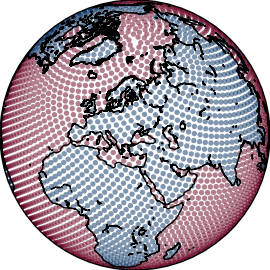
Here is what this looks like on a controlled synthetic task, a checkerboard pattern painted uniformly on a sphere via a Fibonacci lattice:

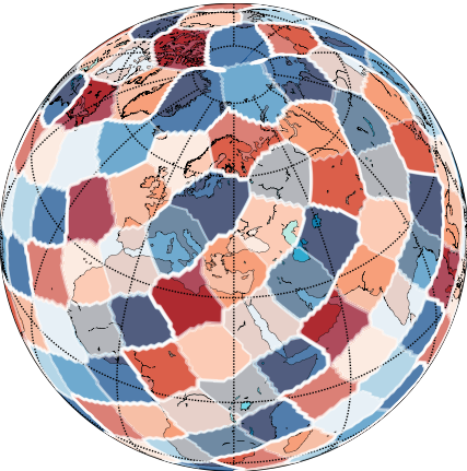
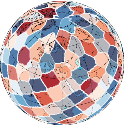
**FcNet(SH):** clean, artifact-free prediction across the entire globe, including both poles

**FcNet(Grid):** prominent artifacts radiate from the North Pole, a direct consequence of the rectangular domain assumption

The left image uses Spherical Harmonic embeddings. The right uses Grid (a DFS variant). Same neural network, same data, same training protocol. The only difference is the positional encoding, and the polar artifacts are immediately visible.

This is not a cosmetic blemish. In any application where high-latitude predictions matter (Arctic sea ice, Antarctic biodiversity, polar climate dynamics) these artifacts are systematic errors in the region of greatest scientific interest.

Spherical Harmonics: The Right Basis for a Sphere

The Core Idea

Spherical Harmonics (SH) are orthogonal basis functions defined natively on the surface of a sphere. They are the spherical analogue of Fourier series: just as sines and cosines decompose a periodic signal on a line, spherical harmonics decompose a signal on a sphere.

Any square-integrable function on \(S^2\) can be written as:

\[ f(\lambda,\phi) = \sum_{l=0}^{\infty}\sum_{m=-l}^{l} w_l^m \; Y_l^m(\lambda,\phi) \]

\(Y_l^m\) is the harmonic of degree \(l\) and order \(m\)
\(w_l^m\) are scalar coefficients (learnable weights in our context)
Degree \(l\) controls spatial frequency: \(l=0\) is a uniform field, \(l=1\) captures hemispheric contrasts, \(l=2\) introduces quadrupolar patterns, and so on
Order \(m\) (with \(|m|\leq l\)) controls the rotational orientation of each pattern

In practice we truncate at a maximum degree \(L\), yielding \(L^2\) basis functions. The choice of \(L\) directly governs the finest angular resolution the embedding can represent.

Spherical harmonics appear everywhere in physics because they are the eigenfunctions of the Laplace–Beltrami operator on the sphere, the natural generalization of the Laplacian to curved surfaces. Using them for geographic encoding is not an aesthetic choice; it is a statement that the basis should respect the geometry of the domain.

Visualizing the Decomposition

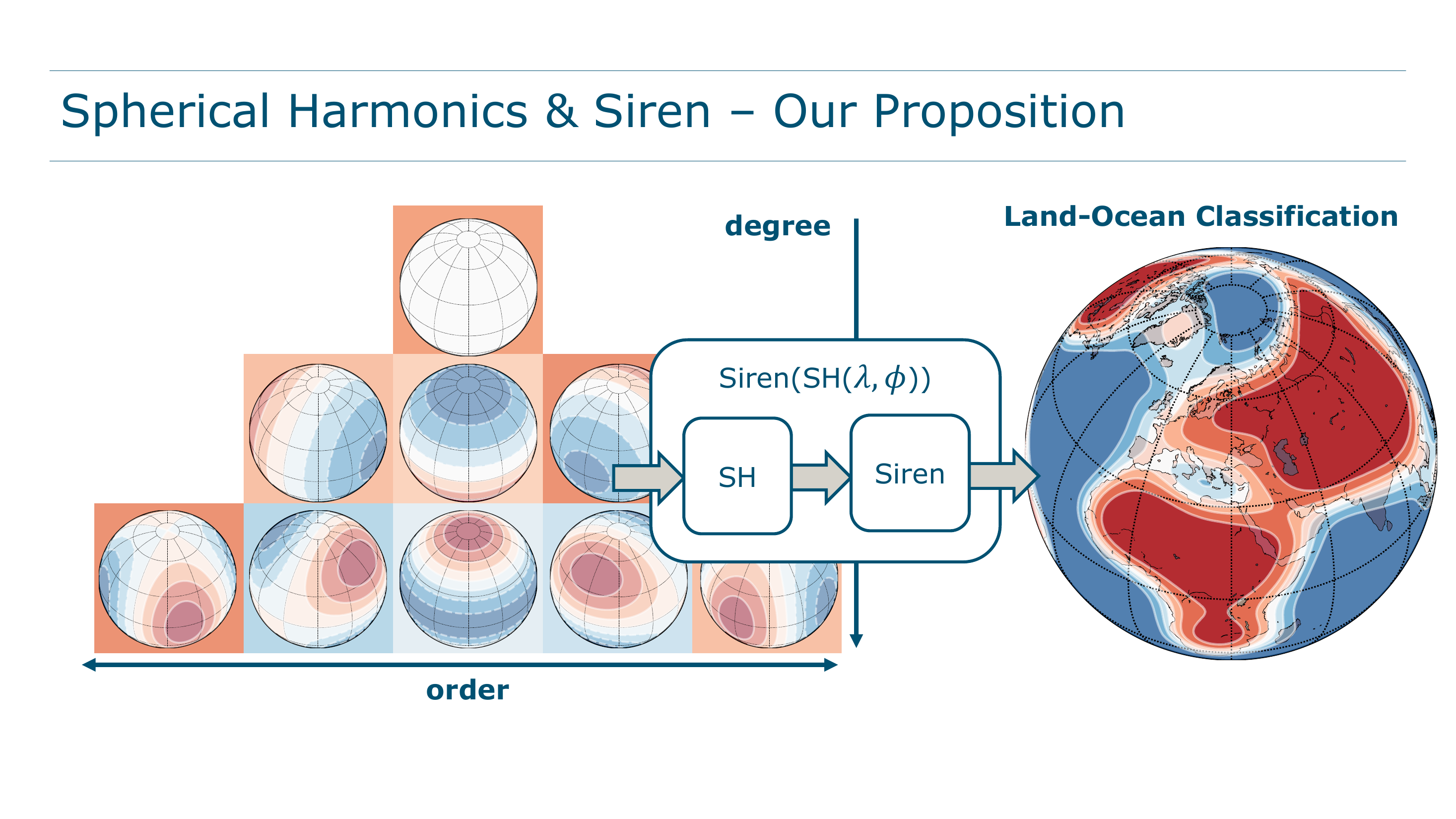
The figure below, from the paper, shows how this works concretely. Individual \(Y_l^m\) basis functions (bottom-left) capture patterns at different angular scales. A triangular weight matrix (top-left) stores the learned coefficients (triangular because \(|m|\leq l\)). The weighted sum (right) reconstructs the target function, here a land-ocean mask:

**Weighted Spherical Harmonics as a location encoder.** With just \(L=3\) (nine basis functions and nine learnable weights), the model already captures the broad continental layout. No hidden layers, no nonlinearities, just a linear combination of the right building blocks.

Nine parameters. Nine basis functions. Already a recognizable outline of Earth’s continents. That is the power of choosing a basis matched to the geometry.

The Real-Valued Form

Each harmonic is computed from normalized associated Legendre polynomials \(\bar{P}_l^m\):

\[ Y_{l,m}(\lambda,\phi) = \begin{cases} (-1)^m\sqrt{2}\;\bar{P}_l^{|m|}(\cos\lambda)\sin(|m|\phi), & m<0\\[4pt] \bar{P}_l^m(\cos\lambda), & m=0\\[4pt] (-1)^m\sqrt{2}\;\bar{P}_l^m(\cos\lambda)\cos(m\phi), & m>0 \end{cases} \]

The Legendre polynomials are constructed by recursive differentiation and can be pre-computed analytically using symbolic algebra (SymPy), then compiled into efficient GPU kernels via PyTorch JIT. This engineering detail matters. See the efficiency section below.

The crucial mathematical property: orthogonality. Each \(Y_l^m\) is independent of every other. Adjusting the weight of one harmonic does not interfere with learning another. And because the functions are defined intrinsically on \(S^2\), there are no singularities, no coordinate chart boundaries, and no artifacts at the poles.

From Continents to Coastlines: Resolution Control

How does increasing \(L\) affect the encoding? The following figures answer this directly on the land-ocean classification task.

With a linear layer (i.e., \(y = \mathbf{w}^\top\text{SH}(\lambda,\phi)\), just weighted summation):

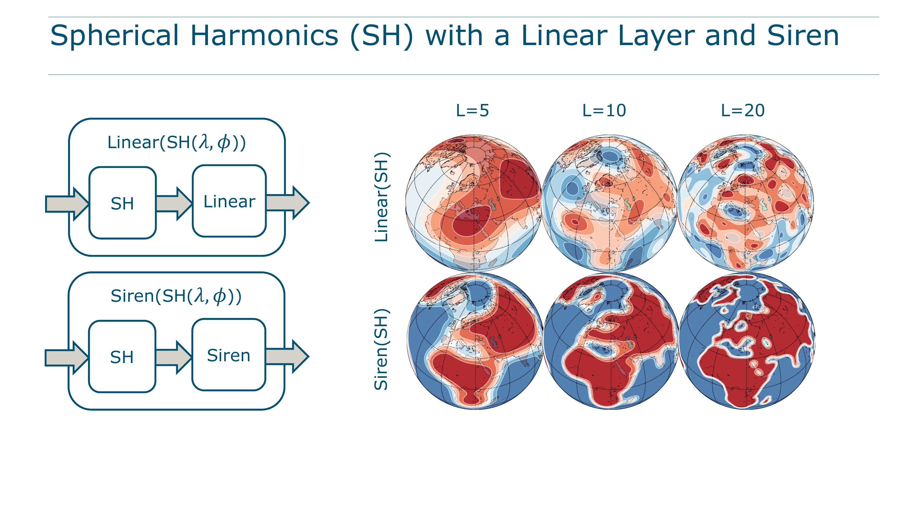
**Siren(SH) with increasing L:** neural network recovers detail far beyond what the raw harmonics offer alone

The maximum resolvable spatial frequency of the linear model is analytically determined:

\[ f^{\max} = \frac{180°}{2L} \]

At \(L=10\), the model can resolve ~9° features. At \(L=20\), ~4.5°. Replacing the linear layer with a SirenNet roughly doubles the effective resolution at the same \(L\), because the network learns to combine harmonics nonlinearly, synthesizing fine detail from coarser basis functions.

This is a key insight: both the embedding and the network contribute to resolution. SH provides geometry-faithful building blocks; the neural network learns how to assemble them into sharp, task-specific maps.

SirenNet: A Neural Network That Learns Its Own Encoding

Architecture

Sinusoidal Representation Networks (SirenNets), introduced by Sitzmann et al. (2020) for implicit neural representations, replace ReLU with the sine function:

\[ \text{SirenNet}(\mathbf{x}) = \sin(\mathbf{W}\mathbf{x} + \mathbf{b}) \]

Each layer is simply: linear projection → dropout → sine activation. No skip connections, no batch normalization. Architecturally simpler than FcNet, yet, as this paper demonstrates for the first time in the location encoding context, remarkably powerful.

The Theoretical Surprise: Siren \(\approx\) Learned DFS

This is the paper’s most elegant theoretical contribution. Consider the Grid positional encoding. Using the identity \(\cos\theta = \sin(\theta + \tfrac{\pi}{2})\), Grid can be rewritten entirely in terms of sine:

\[ \text{Grid}(\lambda,\phi) = \bigcup_{s=0}^{S-1}\Big[\sin\!\big(\tfrac{\lambda}{\alpha_s}+\tfrac{\pi}{2}\big),\;\sin\!\big(\tfrac{\lambda}{\alpha_s}\big),\;\sin\!\big(\tfrac{\phi}{\alpha_s}+\tfrac{\pi}{2}\big),\;\sin\!\big(\tfrac{\phi}{\alpha_s}\big)\Big] \]

Now write out a 1-layer SirenNet applied directly to \((\lambda,\phi)\):

\[ \text{SirenNet}(\lambda,\phi) = \bigcup_{h=1}^{H}\Big[\sin(w_h^\lambda\,\lambda + w_h^\phi\,\phi + b_h)\Big] \]

If you constrain SirenNet’s weights so that each hidden unit processes either longitude or latitude (not both), and fix certain biases to \(0\) or \(\frac{\pi}{2}\), you recover Grid exactly. The difference: in Grid, the frequency scales \(1/\alpha_s\) are hand-designed; in SirenNet, the corresponding weights are learned via gradient descent.

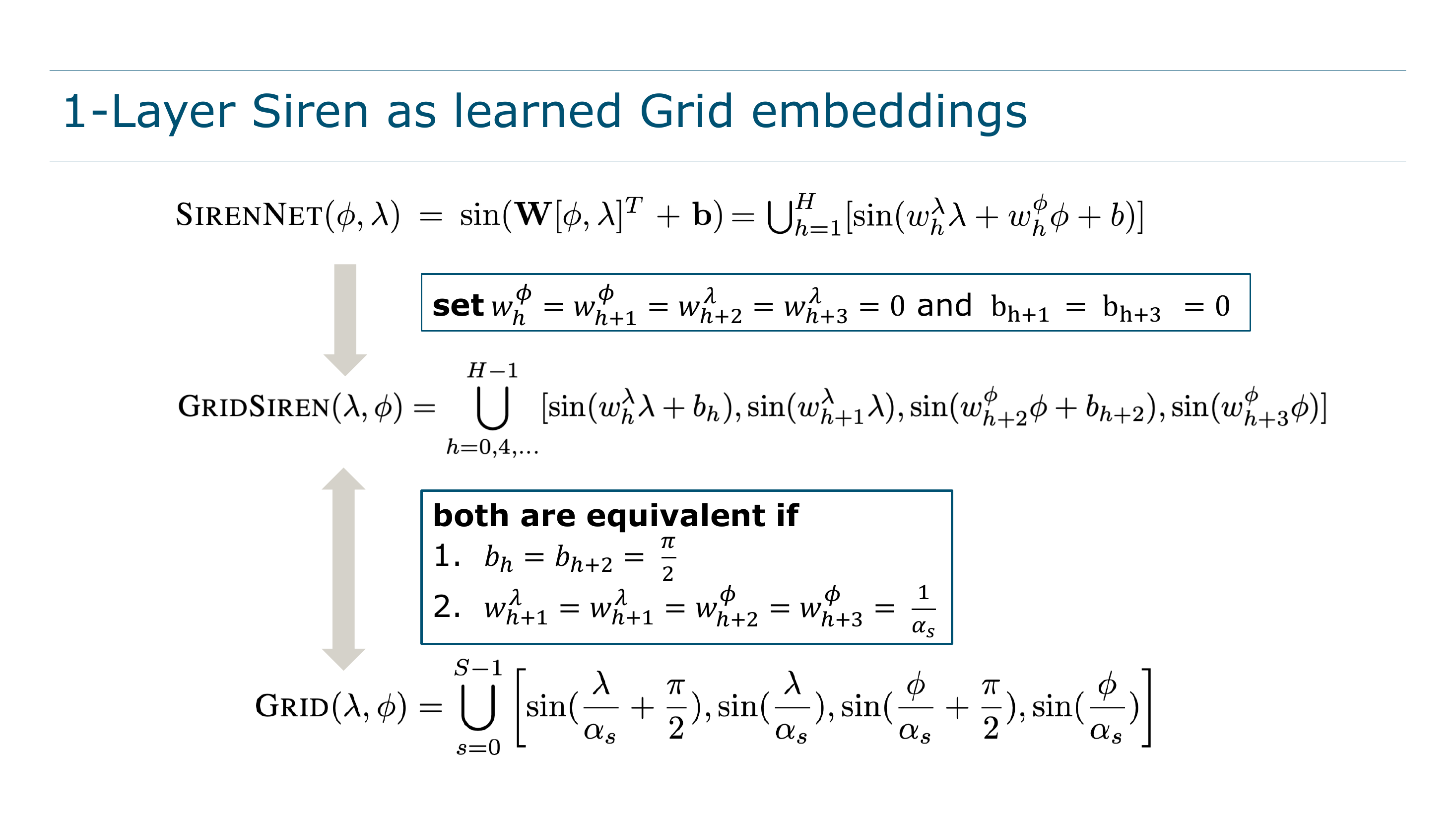
**Slide from the paper presentation:** the analytic correspondence between a 1-layer Siren and Grid-style DFS features. Fixed frequencies become trainable parameters.

Why This Matters

This equivalence dissolves the boundary between positional embedding and neural network. A SirenNet does not merely process a positional encoding: its first layer is a positional encoding, one that adapts its frequency allocation to the task. This explains a surprising empirical finding: SirenNet with raw (Direct) coordinate input is already a strong baseline, because the network learns the encoding it needs.

Why Combine Both?

If SirenNet can learn its own frequency features, why bother with Spherical Harmonics at all?

Because SH provides something SirenNet alone cannot: guaranteed geometric consistency on the sphere. SirenNet’s learned frequencies still operate on the raw \((\lambda,\phi)\) parameterization, inheriting its polar singularities. Spherical Harmonics are defined intrinsically on \(S^2\) with no singularities, no chart boundaries, and uniform behavior from equator to pole.

The combination (Siren(SH)) gives both: geometry-faithful basis functions and adaptive nonlinear frequency mixing. The SH embedding guarantees global consistency; the SirenNet wrings maximum resolution and task-specific expressivity from those harmonics.

Experimental Design

The paper evaluates every combination of 10 positional embeddings \(\times\) 3 neural networks across 4 tasks. This \(10 \times 3 \times 4\) design is a significant strength: it prevents cherry-picking favorable PE-NN-task combinations and reveals systematic patterns about what works and why.

The Four Tasks

**Checkerboard:** A Fibonacci-lattice pattern on the sphere with 16 classes. Synthetic, controlled, and maximally diagnostic: any polar artifact shows up immediately.

**Land-Ocean:** Binary classification using Natural Earth shapefiles. Spans scales from continents to small islands, with evaluation points covering the full globe.

**ERA5 Climate Interpolation:** Eight continuous variables (temperature, wind components, pressure, humidity, radiation, precipitation) learned jointly from just 1% of the global ERA5 reanalysis grid. A demanding multi-task regression.

**iNaturalist 2018:** Location-enhanced image classification for 8,142 species. The location encoder outputs \(P(y|\lambda,\phi)\), which multiplies with a fixed InceptionV3 image classifier \(P(y|I)\).

Each task probes a different facet of location encoding: polar behavior (Checkerboard), multi-scale shape recovery (Land-Ocean), multi-channel physical signal interpolation (ERA5), and real-world utility under geographic sampling bias (iNaturalist).

Results

Checkerboard Classification

Accuracy (%) on the Fibonacci-lattice checkerboard. Means and standard deviations over 5 runs.
Positional Embedding	Linear	FcNet	SirenNet
Direct	8.1 \(\pm\) 0.3	30.0 \(\pm\) 11.2	94.7 \(\pm\) 0.1
Cartesian3D	8.5 \(\pm\) 0.4	85.5 \(\pm\) 1.2	95.7 \(\pm\) 0.2
Grid	10.5 \(\pm\) 0.6	93.5 \(\pm\) 0.3	93.7 \(\pm\) 0.4
SphereC+	23.5 \(\pm\) 0.6	93.7 \(\pm\) 0.4	94.4 \(\pm\) 0.1
SH	94.8 \(\pm\) 0.1	94.9 \(\pm\) 0.1	95.8 \(\pm\) 0.0

Two patterns stand out:

SH is the only embedding that performs excellently regardless of network complexity. Even with a bare linear layer (no hidden units, no nonlinearity), SH reaches 94.8%, a number that most other embeddings need a full SirenNet to approach. When the basis is good enough, the downstream model barely matters.
SirenNet is the only network that performs well regardless of embedding quality. Even with Direct coordinates (just raw \(\lambda,\phi\)), SirenNet reaches 94.7%. When the network can learn its own encoding, the upstream PE barely matters.

The combination of both (Siren(SH) at 95.8%) is best overall.

Land-Ocean Classification

Accuracy (%) on land-ocean classification.
PE	Linear	FcNet	SirenNet
Direct	71.4 \(\pm\) 0.0	90.3 \(\pm\) 0.7	95.1 \(\pm\) 0.3
Grid	81.7 \(\pm\) 0.1	95.1 \(\pm\) 0.1	95.5 \(\pm\) 0.2
SphereC+	84.6 \(\pm\) 0.2	95.3 \(\pm\) 0.1	95.5 \(\pm\) 0.1
SH	94.4 \(\pm\) 0.1	95.9 \(\pm\) 0.1	95.8 \(\pm\) 0.1

The same story holds. The gap between SH-Linear (94.4%) and Grid-Linear (81.7%) is a 13-point jump, purely from changing the basis functions. FcNet(SH) edges out as the top single score at 95.9%.

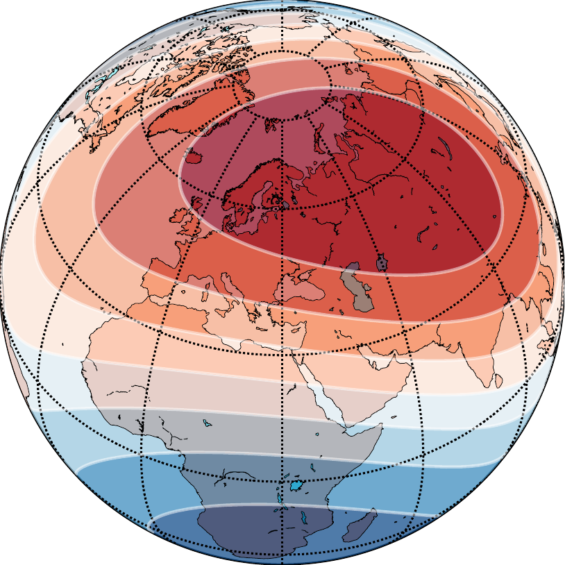
ERA5 Climate Interpolation

Mean Squared Error for 8-variable ERA5 interpolation (lower is better). 10 runs.
PE	Linear	FcNet	SirenNet
Direct	27.19 \(\pm\) 0.08	7.83 \(\pm\) 1.06	1.62 \(\pm\) 0.10
Grid	9.83 \(\pm\) 0.01	1.51 \(\pm\) 0.04	2.37 \(\pm\) 0.13
SphereC+	8.50 \(\pm\) 0.02	1.38 \(\pm\) 0.03	1.97 \(\pm\) 0.08
SH	1.39 \(\pm\) 0.02	0.58 \(\pm\) 0.02	1.19 \(\pm\) 0.04

This is where geometry-faithful encoding pays off most dramatically. FcNet(SH) at 0.58 more than halves the error of the next best competitor (SphereC+ at 1.38), a 58% reduction.

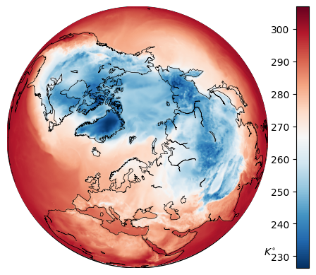
Why such a large gap? ERA5 interpolation requires learning eight coupled physical fields simultaneously from sparse (1%) observations spanning the entire globe, including polar regions. A geometry prior that distorts at high latitudes compounds errors across all eight channels. SH’s native spherical support avoids this compounding entirely.

Predicting temperature from scattered stations is hard. Predicting temperature, wind speed, humidity, pressure, radiation and precipitation jointly from 1% of the data is much harder. Every geometric error in the encoding now propagates through eight correlated targets. This is precisely where a principled spherical basis earns its keep.

iNaturalist 2018

Image-only baselines: 59.2% top-1, 77.0% top-3.

Relative accuracy improvement from adding location to an InceptionV3 image classifier.
Method	Top-1 gain	Top-3 gain
FcNet(Direct)	+9.3 \(\pm\) 0.3	+7.1 \(\pm\) 0.2
FcNet(SphereM+)	+12.0 \(\pm\) 0.1	+8.4 \(\pm\) 0.1
Siren(Direct)	+12.1 \(\pm\) 0.1	+8.8 \(\pm\) 0.1
Siren(SphereC)	+12.3 \(\pm\) 0.1	+8.8 \(\pm\) 0.1
Siren(SH)	+12.3 \(\pm\) 0.2	+9.0 \(\pm\) 0.1

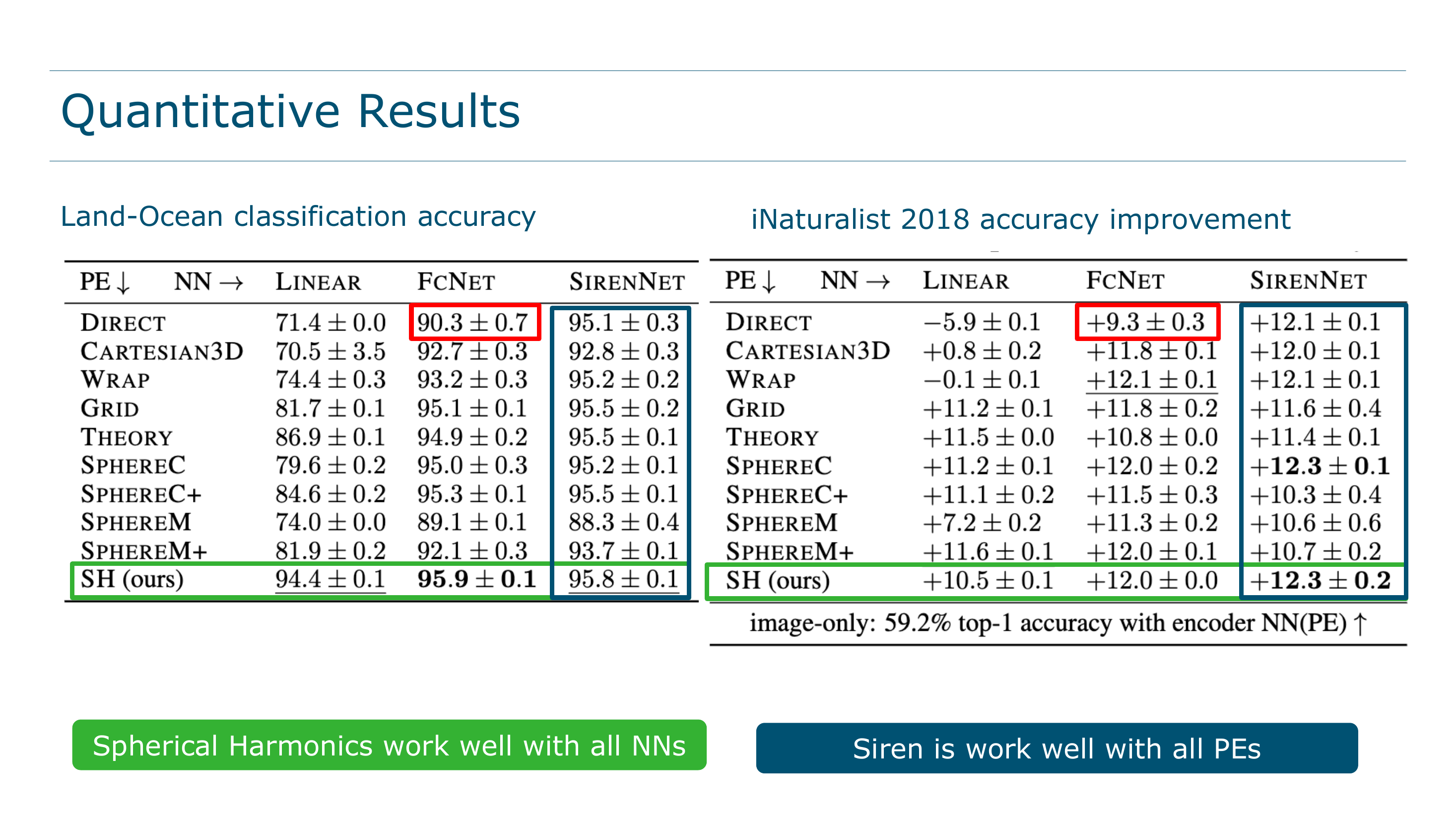
Full result summary from the paper presentation

Siren(SH) is tied for best top-1 and clearly best on top-3. The margins are tighter here than on ERA5, which the paper attributes to iNaturalist’s geographic sampling bias: most observations come from the US and Europe, with sparse coverage at high latitudes where SH’s advantages are most pronounced. In aggregate metrics dominated by mid-latitude data, the polar advantage shows up less, but it still matters for the species that actually live near the poles.

The Polar Story

This is arguably the most important analysis in the paper: a latitude-by-latitude breakdown of prediction quality.

Accuracy by Latitude Band

The checkerboard task is split into 20° latitude bands. Classification accuracy is measured separately in each band:

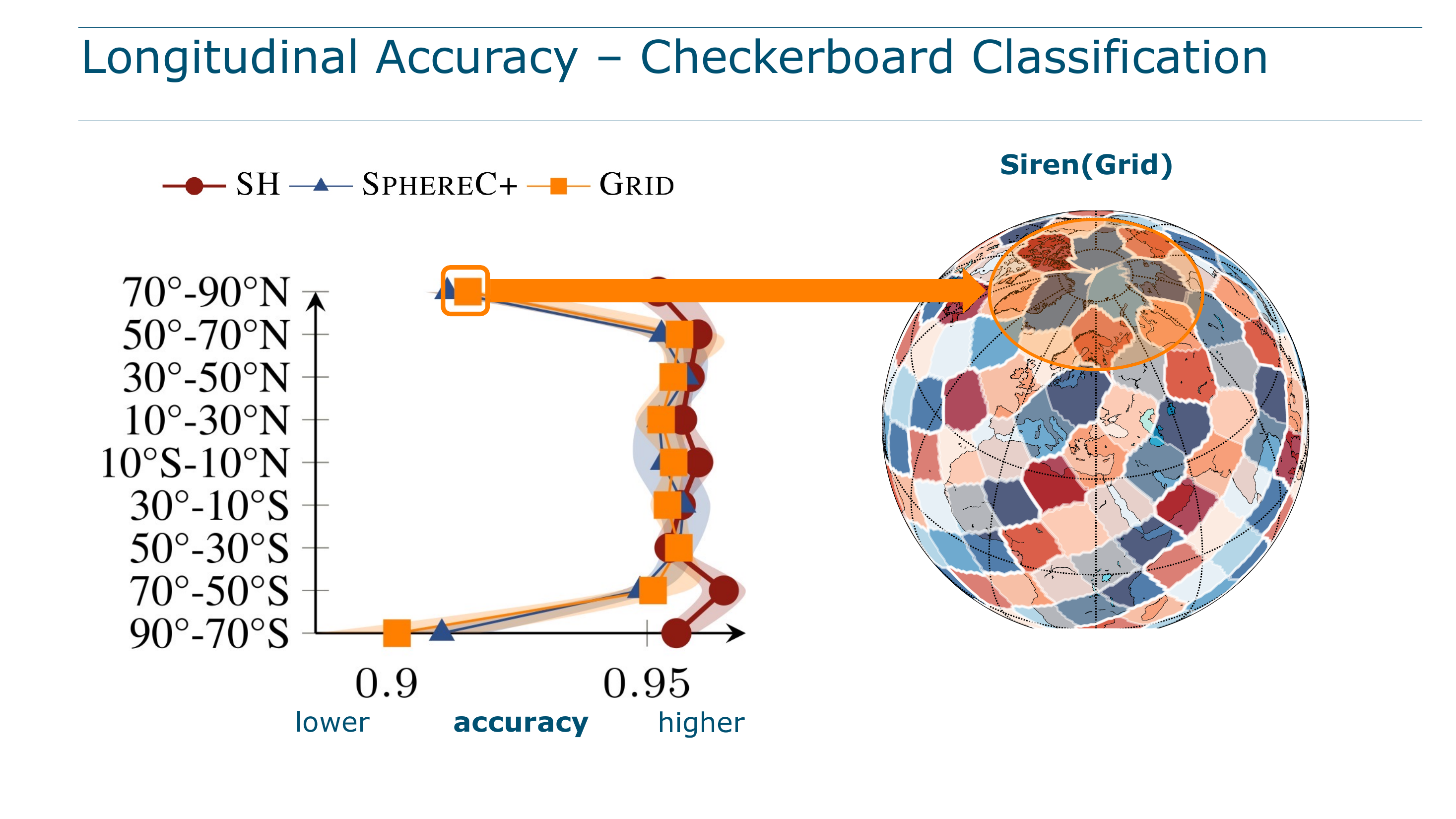
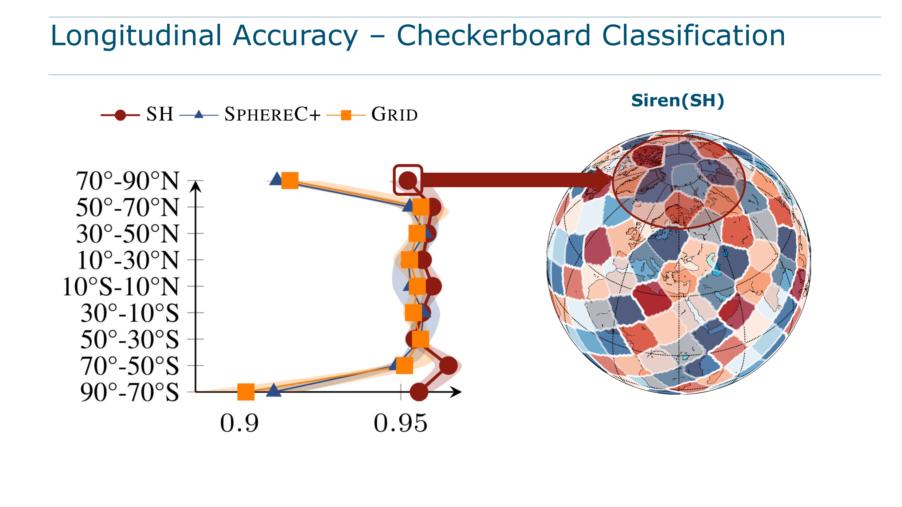
**DFS-style encodings (Grid, SphereC+):** clear accuracy degradation above 70° latitude in both hemispheres, regardless of the neural network

**Spherical Harmonics:** stable accuracy from equator to pole. The encoding introduces no geometric distortion at any latitude.

The degradation of DFS methods at 70–90° is not subtle. It is a visible, consistent drop. SirenNet helps partially in the 50–70° range by compensating with learned frequencies, but cannot overcome the fundamental singularity of the planar chart at the poles. Only SH maintains uniform performance everywhere.

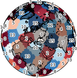
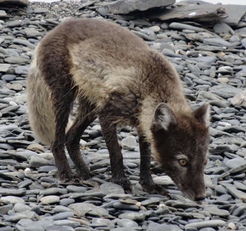
A Real-World Consequence: The Arctic Fox

The latitude-band analysis is quantitative. The Arctic Fox example makes the same point viscerally. Here are learned species distribution maps \(P(y=\text{Arctic Fox}\,|\,\lambda,\phi)\):

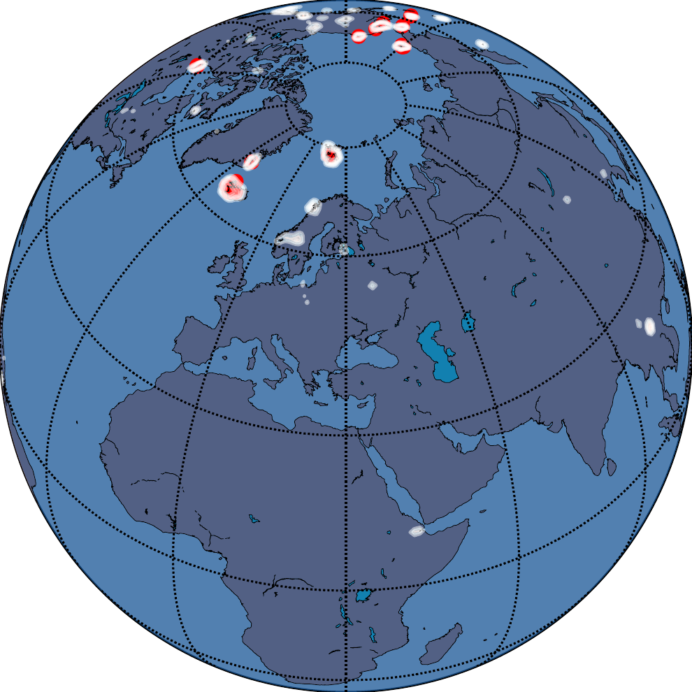
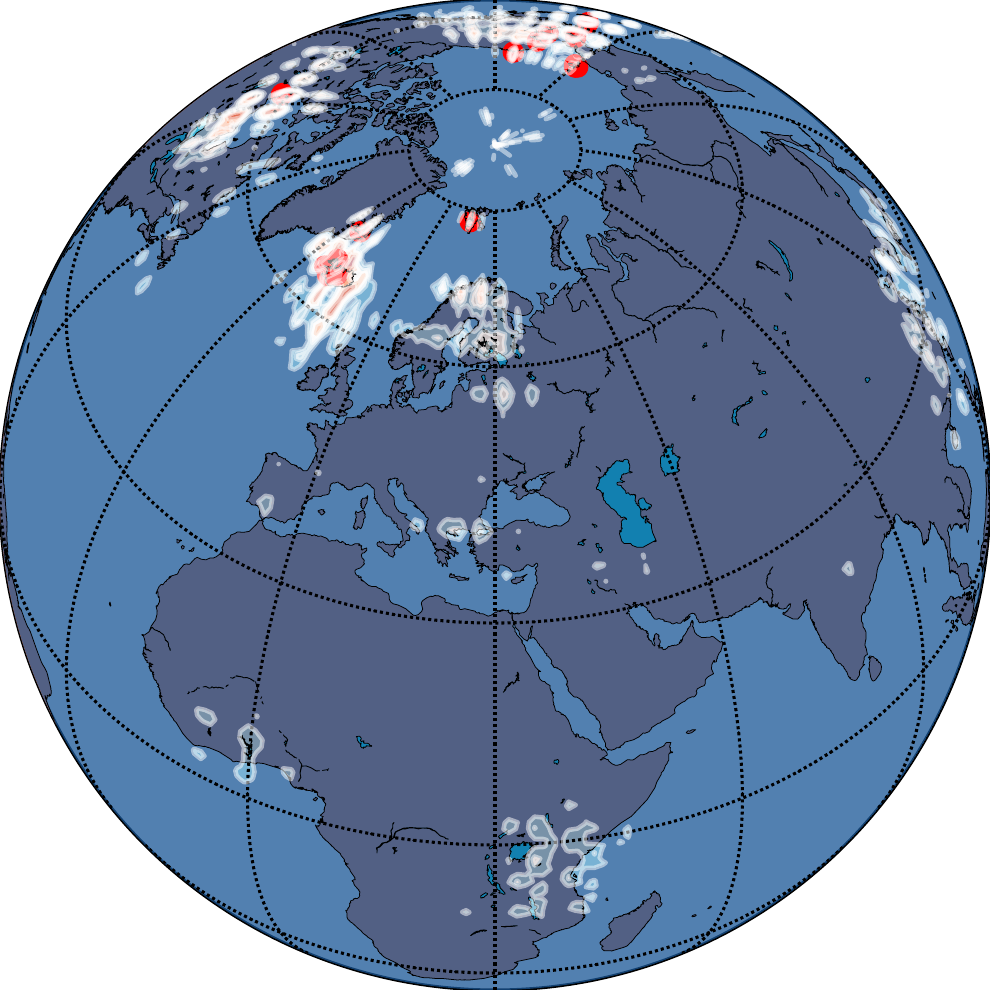
**Siren(SH):** a clean, biologically plausible distribution concentrated in Arctic and sub-Arctic latitudes

**Siren(SphereM+):** vertical meridian artifacts slice through the Arctic, exactly where this species actually lives

The DFS-based encoding produces its worst artifacts in the precise geographic region that defines the Arctic Fox’s habitat. This is not an edge case or a stress test. It is a direct failure on the species’ core range. For conservation biology, ecological forecasting, or any polar-focused application, this is an unacceptable systematic error.

Computational Efficiency

A natural concern: Legendre polynomials and their normalizations sound expensive. Is the accuracy gain worth a computational penalty?

The paper provides a clear answer. A naive closed-form implementation does scale poorly. But the paper’s analytic implementation (which pre-computes each harmonic symbolically using SymPy, simplifies the expressions, and JIT-compiles them) is dramatically faster:

Inference time for 10,000 test points.
\(L\) (SH) / Scales (SphereC+)	SH analytic	SH closed-form	SphereC+
10	0.090 s	0.248 s	0.301 s
20	0.191 s	1.357 s	0.308 s
40	0.994 s	9.846 s	0.319 s

At \(L \leq 20\) (sufficient for most tasks), the analytic SH implementation is actually faster than SphereC+. At \(L=40\), it is about 3\(\times\) slower, but \(L=40\) resolves 2.25° features, which is finer than most applications need, and the absolute runtime (under 1 second for 10,000 points) is entirely practical.

Practical guidance for choosing \(L\):

\(L=10\) (resolves ~9°): continental and global-scale patterns
\(L=20\) (resolves ~4.5°): regional patterns, sufficient for the vast majority of tasks
\(L\geq30\) (resolves ~3° and finer): detailed coastlines, small islands, fine-grained local structure
Adding SirenNet effectively doubles the resolution you get at a given \(L\)

The Full Positional Encoding Landscape

To contextualize the contribution, here is a summary of all ten positional embeddings the paper evaluates:

The ten positional embeddings compared in the paper. \(S\) = number of frequency scales. Only SH is defined intrinsically on \(S^2\).
Encoding	Core Idea	Dimensions	Polar-Safe
Direct	Raw \((\lambda,\phi)\)	2	No
Cartesian3D	Spherical\(\to(x,y,z)\)	3	Partial
Wrap	Single-scale sin/cos	4	No
Grid	Multi-scale sin/cos	\(4S\)	No
Theory	Hexagonal basis	\(6S\)	No
SphereC	Simplified DFS	\(3S\)	No
SphereC+	SphereC + Grid	\(7S\)	No
SphereM	DFS variant	\(5S\)	No
SphereM+	SphereM + Grid	\(9S\)	No
Spherical Harmonics	Native spherical basis	\(L^2\)	Yes

Every DFS-derived method (Grid through SphereM+) applies trigonometric functions to a rectangular parameterization of the sphere. Only Spherical Harmonics bypass the parameterization entirely.

Practical Recommendations

The paper’s results converge on clear guidance:

Decision Matrix

Your Scenario	Recommended Setup
Global data with any polar coverage	Siren(SH)
Climate / environmental regression	FcNet(SH) (best ERA5 score by far)
Quick strong baseline, no PE tuning	Siren(Direct) (the network learns its own encoding)
Maximum interpretability	Linear(SH) (each weight scales one basis function)
Regional mid-latitude data only	Any SirenNet combination works well

The default choice for new projects should be Siren(SH) unless you have a specific reason not to use it.

Limitations and Open Directions

No paper solves everything. Honest limitations noted by the authors and worth flagging:

iNaturalist gains are narrow. The dataset’s heavy geographic bias toward the US and Europe means aggregate metrics underweight polar performance. On a uniformly sampled benchmark, the SH advantage would likely be larger.
Very high SH orders (\(L>40\)) incur nontrivial cost. The analytic implementation helps enormously, but SH does not scale as invariantly as DFS encodings whose runtime is independent of the number of scales.
Spatiotemporal encoding remains open. The paper encodes space (\(\lambda,\phi\)) but not time. Extending SH-type geometric encodings to space-time is a natural and important next step for weather and climate applications.
The SirenNet–DFS equivalence is shown for 1 layer. Multi-layer Siren learns richer features (products of frequencies, phase shifts), and the theoretical characterization of what a deep SirenNet represents is still developing.

These are research opportunities, not refutations. The core thesis (that geographic encoding should respect spherical geometry) is well-supported across every experiment in the paper.

Takeaways

Three ideas to carry away from this paper:

1. Geometry should match the domain. SH basis functions are not exotic; they have been used in geophysics for over 200 years. What is new is recognizing that the same principle applies to neural location encoders. If your data lives on a sphere, your encoding should live on a sphere.

2. The PE–NN boundary is softer than it looks. The analytic result showing 1-layer Siren \(\approx\) learned Grid encoding reframes the entire PE-vs-NN discussion. A SirenNet does not just consume positional features; it generates them. This opens a path toward end-to-end learnable, parameter-efficient encodings.

3. Evaluation should be global. Aggregate accuracy on geographically biased benchmarks can hide severe failures at high latitudes. The latitude-band analysis in this paper should become standard practice for any method claiming to handle global geographic data.